Huygens wavefront tracing: A robust alternative to conventional ray tracing

Gaussian velocity anomalies

Our first two examples are Gaussian velocity anomalies (one positive and one negative) with a magnitude of 2.0 km/s in a constant velocity medium of 2.0 km/s for the positive anomaly, shown in Figure 5, and of 3.0 km/s for the negative anomaly in Figure 6. The anomaly is centered at a depth of 1.0km and has a half-width of 300 m. The source is placed on the surface directly above the anomaly (at x=6.0 km).

gp-velocity
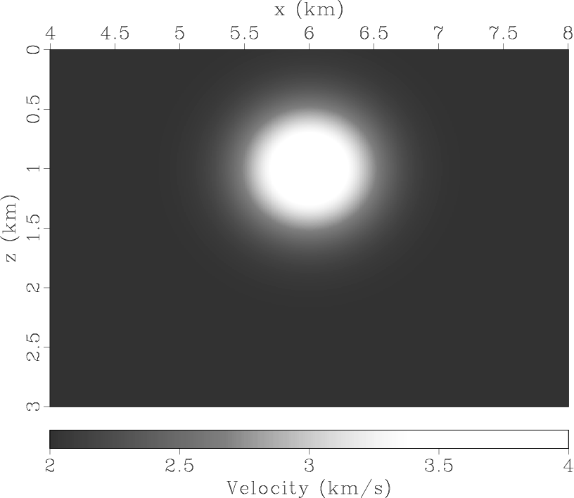
Figure 5. A Gaussian positive velocity anomaly. The background velocity is 2.0 km/s, and the maximum anomaly at the center is +2.0 km/s.

gn-velocity
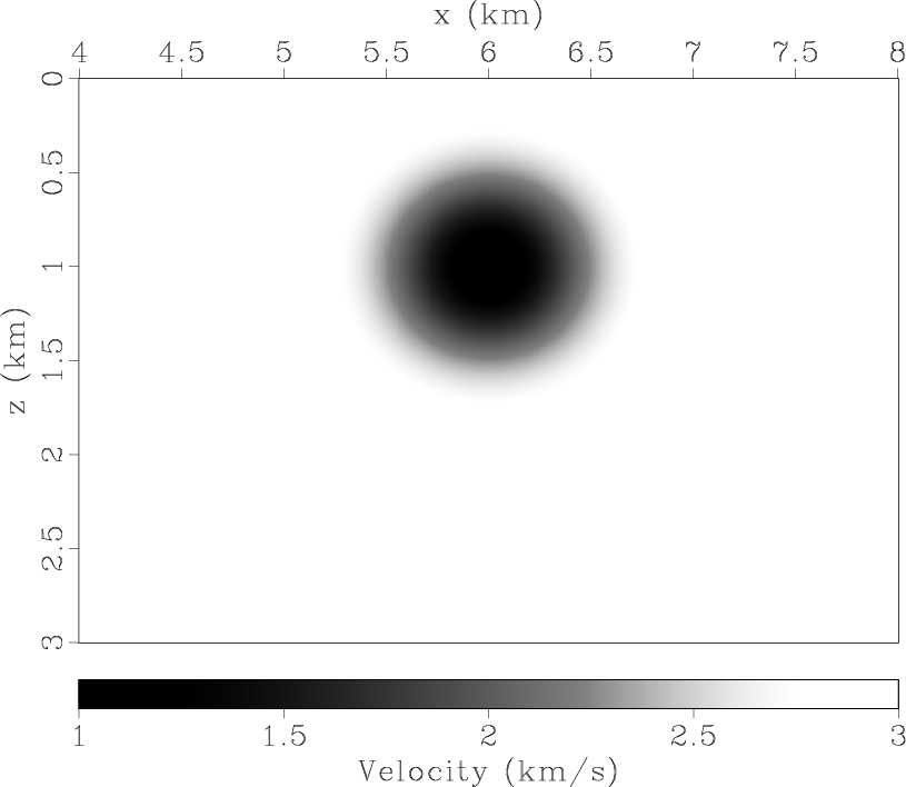
Figure 6. A Gaussian negative velocity anomaly. The background velocity is 3.0 km/s, and the maximum anomaly at the center is -2.0 km/s.

We have selected these velocity models to test the way our method applies to different patterns of velocity variation. In the case of the negative anomaly, the rays focus inward, while in the case of the positive anomaly the rays spread outward.

The distribution of rays as obtained with the PRT and HWT methods are presented in Figure 7 for the positive anomaly, and in Figure 8 for the negative.

gp-velrw
Figure 7. The rays obtained in the case of the Gaussian positive velocity anomaly. We present the rays obtained with the PRT method (left) and with the HWT method (right). The source is located on the surface at x=6.0 km.

gn-velrw
Figure 8. The rays obtained in the case of the Gaussian negative velocity anomaly. We present the rays obtained with the PRT method (left) and with the HWT method (right). The source is located on the surface at x=6.0 km.

One way to compare the two methods is to compute the distance between the points that correspond to the same ray, identified by the same take-off angle, at the same traveltimes. This is obviously not a perfect quantitative comparison, because once two rays, obtained with the two methods, become slightly divergent, they keep going in different directions, and thus the distance between corresponding points keeps growing (Figures 9 and 10). However, this effect is not necessarily a manifestation of decreasing precision. It can be easily seen that if such an angular mismatch doesn't occur, the rays maintain practically the same path (see, for example, the rays shot in the (-20,-40) and (20,40) degree intervals, where the distance decreases in many cases to almost zero). Even in the case of divergent rays, the distance is kept to a reasonable level (less than 1%). Consequently, we do not interpret these differences as error.

gp-diff Figure 9. The distance between the corresponding points on the rays obtained with the PRT method and with the HWT method. Distances are given in meters.

gn-diff Figure 10. The distance between the corresponding points on the rays obtained with the PRT method and with the HWT method. Distances are given in meters.

Huygens wavefront tracing: A robust alternative to conventional ray tracing