 |
 |
 |
 | Modeling 3-D anisotropic fractal media |  |
![[pdf]](icons/pdf.png) |
Next: FORWARD MODELING
Up: RANDOM FIELDS
Previous: Second-order Statistics
The three-dimensional anisotropic von Karman function is given by (Goff and Jordan, 1988):
 |
(4) |
and its three-dimensional Fourier transform is:
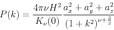 |
(5) |
where
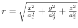 ,
,
 ;
;
 ,
,  and
and  are the characteristic scales of the medium along the
3-dimensions and
are the characteristic scales of the medium along the
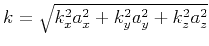
3-dimensions and  ,
,  and
and  are the wavenumber components.
 is the modified Bessel function of order
  ,
where
,
where  is the
Hurst number (Mandelbrot, 1985,1983). The fractal dimension of a stochastic
field characterized by a von Karman autocorrelation is given by:
is the
Hurst number (Mandelbrot, 1985,1983). The fractal dimension of a stochastic
field characterized by a von Karman autocorrelation is given by:
 |
(6) |
where  is the Euclidean dimension i.e.,
  for the three-dimensional problem.
The special case of
for the three-dimensional problem.
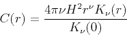
The special case of  yields to the exponential covariance
function that corresponds to a Markov process (Feller, 1971).
yields to the exponential covariance
function that corresponds to a Markov process (Feller, 1971).
 |
(7) |
whose three-dimensional Fourier transform is given by:
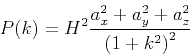 |
(8) |

|
|---|
karman
Figure 1. Comparison of 1-dimensional isotropic von Karman autocorrelation functions for varying hurst number, .
|
|---|
![[png]](icons/viewmag.png) ![[xfig]](icons/xfig.png)
|
|---|
Decreasing the Hurst number, , increases the roughness of the medium.
The limiting cases of unity and zero correspond to a smooth Euclidean random
field and a space-filling field respectively.
Figure 1 shows the one-dimensional isotropic von Karman correlation
function plotted
for different values of . The functions have exponential behavior
but different decay rates.
The higher the slope, the rougher the medium (i.e., the lower is ).
The exponential behavior is explained by the modified Bessel functions
 which in the region
  behave as
 |
(9) |
For comparison of the results, I also include the anisotropic Gaussian
autocovariance function, which in 3-D has the familiar form:
 |
(10) |
and its 3-dimensional Fourier transform is given by:
 |
(11) |
|
|
|
|
| Modeling 3-D anisotropic fractal media | |
|
Next: FORWARD MODELING
Up: RANDOM FIELDS
Previous: Second-order Statistics
2013-03-03