|
 |
 |
 | A second-order fast marching eikonal solver |  |
![[pdf]](icons/pdf.png) |
Next: Accuracy
Up: Rickett & Fomel: Second-order
Previous: Introduction
Under a high frequency approximation, propagating wavefronts may be
described by the eikonal equation,
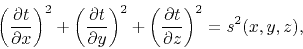 |
(1) |
where  is the traveltime,
  is the slowness, and
  ,
,  and
and  represent the spatial Cartesian coordinates.
The fast marching method solves equation (1) by
directly mimicking the advancing wavefront.
Every point on the computational
grid is classified into three groups:
points behind the wavefront, whose traveltimes are known and fixed;
points on the wavefront, whose traveltimes have been calculated, but
are not yet fixed; and points ahead of the wavefront.
The algorithm then proceeds as follows:
- Choose the point on the wavefront with the smallest traveltime.
- Fix this traveltime.
- Advance the wavefront, so that this point is behind it, and
adjacent points are either on the wavefront or behind it.
- Update traveltimes for adjacent points on the wavefront by
solving equation (1) numerically.
- Repeat until every point is behind the wavefront.
The update procedure (step 4.) requires the solution of the following
quadratic equation for ,
where  is a backward difference operator at
grid point,
is a backward difference operator at
grid point,  ,
,  is a forward operator, and
finite-difference operators in and are defined similarly.
The roots of the quadratic equation,
is a forward operator, and
finite-difference operators in and are defined similarly.
The roots of the quadratic equation,
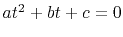 ,
can be calculated explicitly as
,
can be calculated explicitly as
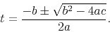 |
(3) |
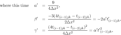
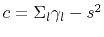
Solving equation (2) amounts to accumulating
coefficients  ,
,  and
and  from its non-zero terms, and evaluating
with equation (3).
from its non-zero terms, and evaluating
with equation (3).
If we choose a two-point finite-difference operator, such as
where
 ,
,
 and
and
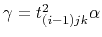 .
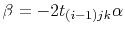
Coefficients , and can now be calculated from
.
Coefficients , and can now be calculated from
 ,
,
 , and
, and
 ,
where the summation index,
,
where the summation index,  , refers to the six terms in
equation (2) subject to the various min/max
conditions.
, refers to the six terms in
equation (2) subject to the various min/max
conditions.
This two-point stencil, however, is only accurate to first-order.
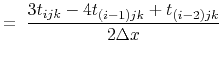
If instead we choose a suitable three-point finite-difference
stencil, we may expect the method to have second-order accuracy. For
example, the second-order upwind stencil,
Coefficients, , and can be accumulated from  ,
,
 and
and  as before, and if the traveltime,
  is not available, first-order values may be substituted.
|
|
|
|
| A second-order fast marching eikonal solver | |
|
Next: Accuracy
Up: Rickett & Fomel: Second-order
Previous: Introduction
2013-03-03