|
|
|
|
The Wilson-Burg method of spectral factorization with application to helical filtering |
We chose an environmental dataset (Claerbout, 2002) for a simple illustration of smooth data regularization. The data were collected on a bottom sounding survey of the Sea of Galilee in Israel (Ben-Avraham et al., 1990). The data contain a number of noisy, erroneous and inconsistent measurements, which present a challenge for the traditional estimation methods (Fomel and Claerbout, 1995).
Figure 9 shows the data after a nearest-neighbor binning
to a regular grid. The data were then passed to an interpolation
program to fill the empty bins. The results (for different values of
![]() ) are shown in Figures 10 and 11.
Interpolation with the minimum-phase Laplacian (
) are shown in Figures 10 and 11.
Interpolation with the minimum-phase Laplacian (![]() ) creates a
relatively smooth interpolation surface but plants artificial
``hills'' around the edge of the sea. This effect is caused by large
gradient changes and is similar to the sidelobe effect in the
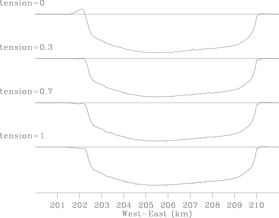
one-dimensional example (Figure 5). It is clearly seen in
the cross-section plots in Figure 11. The abrupt
gradient change is a typical case of a shelf break. It is caused by a
combination of sedimentation and active rifting. Interpolation with
the helix derivative (
) creates a
relatively smooth interpolation surface but plants artificial
``hills'' around the edge of the sea. This effect is caused by large
gradient changes and is similar to the sidelobe effect in the
one-dimensional example (Figure 5). It is clearly seen in
the cross-section plots in Figure 11. The abrupt
gradient change is a typical case of a shelf break. It is caused by a
combination of sedimentation and active rifting. Interpolation with
the helix derivative (![]() ) is free from the sidelobe
artifacts, but it also produces an undesirable non-smooth behavior in
the middle part of the image. As in the one-dimensional example,
intermediate tension allows us to achieve a compromise: smooth
interpolation in the middle and constrained behavior at the sides of
the sea bottom.
) is free from the sidelobe
artifacts, but it also produces an undesirable non-smooth behavior in
the middle part of the image. As in the one-dimensional example,
intermediate tension allows us to achieve a compromise: smooth
interpolation in the middle and constrained behavior at the sides of
the sea bottom.
|
mesh
Figure 9. The Sea of Galilee dataset after a nearest-neighbor binning. The binned data is used as an input for the missing data interpolation program. |

|
|---|---|
|
|

|
|---|
|
gal
Figure 10. The Sea of Galilee dataset after missing data interpolation with helical preconditioning. Different plots correspond to different values of the tension parameter. An east-west derivative filter was applied to illuminate the surface. |
|
|
|
|---|
|
cross
Figure 11. Cross-sections of the Sea of Galilee dataset after missing-data interpolation with helical preconditioning. Different plots correspond to different values of the tension parameter. |
|
|
|
|
|
|
The Wilson-Burg method of spectral factorization with application to helical filtering |