 |
 |
 |
 | The Wilson-Burg method of spectral factorization
with application to helical filtering |  |
![[pdf]](icons/pdf.png) |
Next: Finite differences and spectral
Up: Application of spectral factorization:
Previous: Application of spectral factorization:
The traditional minimum-curvature criterion implies seeking a
two-dimensional surface  in region
  , which corresponds to
the minimum of the Laplacian power:
, which corresponds to
the minimum of the Laplacian power:
 |
(4) |
where  denotes the Laplacian operator:
 .
.
Alternatively, we can seek
as the solution of the biharmonic
differential equation
 |
(5) |
Fung (1965) and Briggs (1974) derive
equation (5) directly from (4) with the help of
the variational calculus and Gauss's theorem.
Formula (4) approximates the strain energy of a thin
elastic plate (Timoshenko and Woinowsky-Krieger, 1968). Taking tension into account modifies
both the energy formula (4) and the corresponding
equation (5). Smith and Wessel (1990) suggest the
following form of the modified equation:
![$\displaystyle \left[(1-\lambda) (\nabla^2)^2 - \lambda (\nabla^2)\right] f(x,y) = 0\;,$](img46.png) |
(6) |
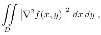
where the tension parameter  ranges from 0 to 1. The
corresponding energy functional is
ranges from 0 to 1. The
corresponding energy functional is
![$\displaystyle \iint\limits_{D} \left[(1-\lambda)\,\left\vert\nabla^2 f(x,y)\right\vert^2 \;+\; \lambda\,\left\vert\nabla f(x,y)\right\vert^2\right]\,dx\,dy\;.$](img47.png) |
(7) |
Zero tension leads to the biharmonic equation (5) and
corresponds to the minimum curvature construction. The case of
 corresponds to infinite tension. Although infinite tension
is physically impossible, the resulting Laplace equation does have the
physical interpretation of a steady-state temperature distribution. An
important property of harmonic functions (solutions of the Laplace
equation) is that they cannot have local minima and maxima in the free
regions. With respect to interpolation, this means that, in the case
of
, the interpolation surface will be constrained to have
its local extrema only at the input data locations.
corresponds to infinite tension. Although infinite tension
is physically impossible, the resulting Laplace equation does have the
physical interpretation of a steady-state temperature distribution. An
important property of harmonic functions (solutions of the Laplace
equation) is that they cannot have local minima and maxima in the free
regions. With respect to interpolation, this means that, in the case
of
, the interpolation surface will be constrained to have
its local extrema only at the input data locations.
Norman Sleep (2000, personal communication) points out that if the
tension term
 is written in the form
 , we can follow an analogy with heat flow and
electrostatics and generalize the tension parameter
to a
local function depending on
, we can follow an analogy with heat flow and
electrostatics and generalize the tension parameter
to a
local function depending on  and
and  . In a more general form,
could be a tensor allowing for an anisotropic smoothing in
some predefined directions similarly to the steering-filter method
(Clapp et al., 1998).
. In a more general form,
could be a tensor allowing for an anisotropic smoothing in
some predefined directions similarly to the steering-filter method
(Clapp et al., 1998).
To interpolate an irregular set of data values,  at points
 , we need to solve equation (6) under the
constraint
, we need to solve equation (6) under the
constraint
 |
(8) |
We can accelerate the solution by recursive filter preconditioning. If
 is the discrete filter representation of the differential
operator in equation (6) and we can find a minimum-phase
filter
is the discrete filter representation of the differential
operator in equation (6) and we can find a minimum-phase
filter
 whose autocorrelation is equal to
, then
an appropriate preconditioning operator is a recursive inverse
filtering with the filter
. The preconditioned formulation
of the interpolation problem takes the form of the least-squares system
(Claerbout, 2002)
whose autocorrelation is equal to
, then
an appropriate preconditioning operator is a recursive inverse
filtering with the filter
. The preconditioned formulation
of the interpolation problem takes the form of the least-squares system
(Claerbout, 2002)
 |
(9) |
where
 represents the vector of known data,
 is
the operator of selecting the known data locations, and
is
the operator of selecting the known data locations, and
 is
the preconditioned variable:
is
the preconditioned variable:
 . After
obtaining an iterative solution of system (9), we
reconstruct the model
. After
obtaining an iterative solution of system (9), we
reconstruct the model
 by inverse recursive filtering:
 . Formulating the problem in
helical coordinates (Mersereau and Dudgeon, 1974; Claerbout, 1998) enables both the spectral
factorization of
and the inverse filtering with
.
. Formulating the problem in
helical coordinates (Mersereau and Dudgeon, 1974; Claerbout, 1998) enables both the spectral
factorization of
and the inverse filtering with
.
|
|
|
|
| The Wilson-Burg method of spectral factorization
with application to helical filtering | |
|
Next: Finite differences and spectral
Up: Application of spectral factorization:
Previous: Application of spectral factorization:
2014-02-15