|
|
|
|
Inverse B-spline interpolation |
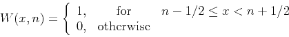
The two simplest forms of the forward interpolation operators are the
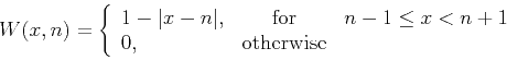
1-point nearest neighbor interpolation with the weight

|
|---|
|
nnint
Figure 1. Nearest neighbor interpolant (left) and its spectrum (right). |
|
|

|
|---|
|
linint
Figure 2. Linear interpolant (left) and its spectrum (right). |
|
|
On the other side of the accuracy scale, there is the infinitely long
sinc interpolant:

|
|---|
|
sincint
Figure 3. Sinc interpolant (left) and its spectrum (right). |
|
|
Several approaches exist for extending the nearest neighbor and linear
interpolation to more accurate (albeit more expensive) methods. One
example is the 4-point cubic convolution suggested by Keys (1981).
The cubic convolution interpolant is a local piece-wise cubic
function, which approximates the ideal sinc equation (4).
Another popular approach is to taper the ideal sinc function in a
local window. For example, one can use the Kaiser window (Kaiser and Shafer, 1980)
I compare the accuracy of different forward interpolation methods on a one-dimensional signal shown in Figure 4. The ideal signal has an exponential amplitude decay and a quadratic frequency increase from the center towards the edges. It is sampled at a regular 50-point grid and interpolated to 500 regularly sampled locations. The interpolation result is compared with the ideal one. Observing Figures 5, 6, and 7, we can see the interpolation error steadily decreasing as we go subsequently from 1-point nearest neighbor to 2-point linear, 4-point cubic convolution, and 8-point windowed sinc interpolation. At the same time, the cost of interpolation grows proportionally to the interpolant length.
|
chirp
Figure 4. One-dimensional test signal. Top: ideal. Bottom: sampled at 50 regularly spaced points. The bottom plot is the input in a forward interpolation test. |

|
|---|---|
|
|
|
binlin
Figure 5. Interpolation error of the nearest neighbor interpolant (dashed line) compared to that of the linear interpolant (solid line). |

|
|---|---|
|
|
|
lincub
Figure 6. Interpolation error of the linear interpolant (dashed line) compared to that of the cubic convolution interpolant (solid line). |

|
|---|---|
|
|
|
cubkai
Figure 7. Interpolation error of the cubic convolution interpolant (dashed line) compared to that of the 8-point windowed sinc interpolant (solid line). |

|
|---|---|
|
|
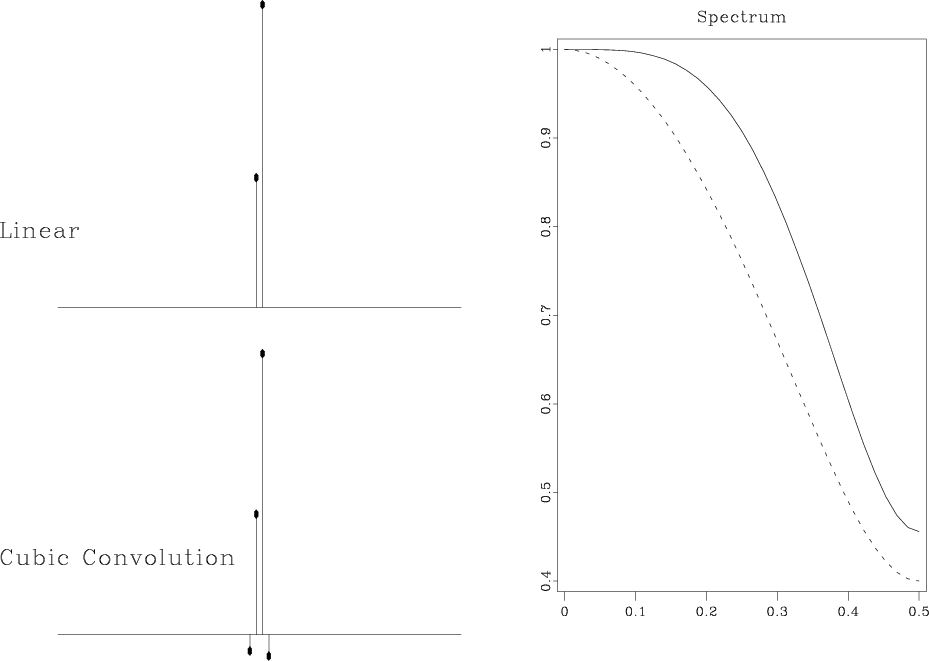
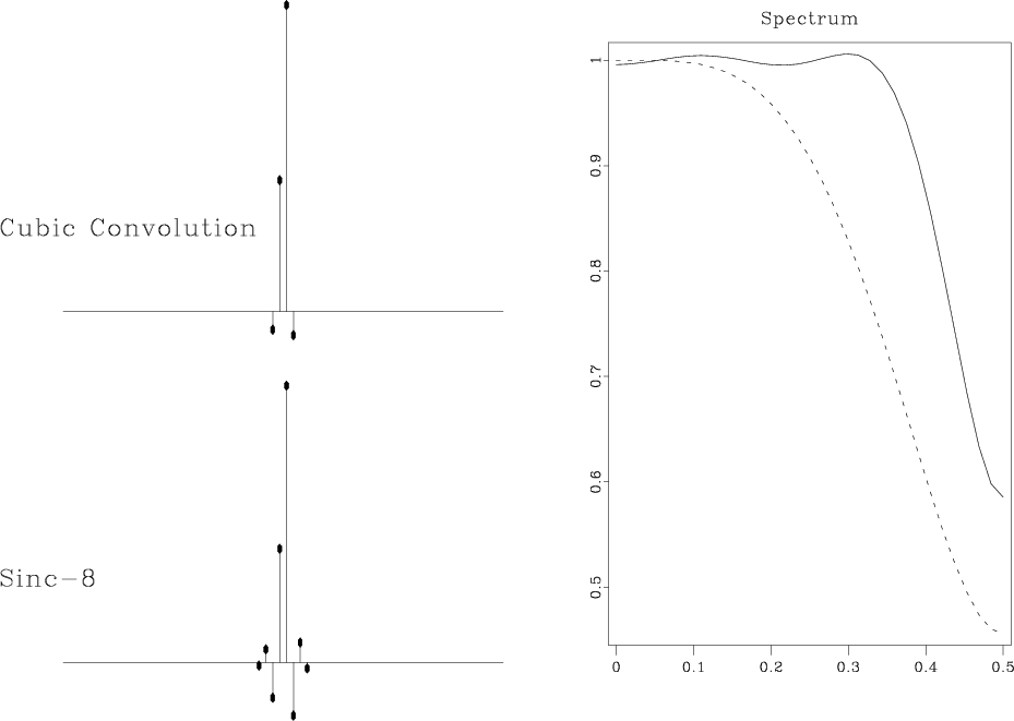
The differences among different methods are also clearly visible from
the discrete spectra of the corresponding interpolants. The left plots
in figures 8 and 9 show discrete
interpolation responses: the function ![]() for a fixed value of
for a fixed value of
![]() . The right plots compare the corresponding discrete spectra. We
can see that the spectrum gets flatter and wider as the accuracy of
the method increases.
. The right plots compare the corresponding discrete spectra. We
can see that the spectrum gets flatter and wider as the accuracy of
the method increases.
|
speclincub
Figure 8. Discrete interpolation responses of linear and cubic convolution interpolants (left) and their discrete spectra (right) for |
|
|---|---|
|
|
|
speccubkai
Figure 9. Discrete interpolation responses of cubic convolution and 8-point windowed sinc interpolants (left) and their discrete spectra (right) for |
|
|---|---|
|
|
|
|
|
|
Inverse B-spline interpolation |
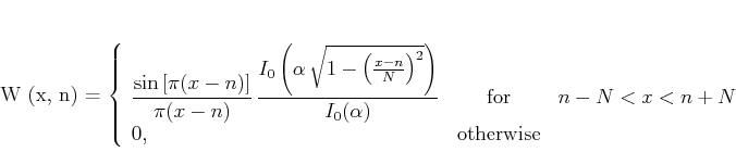
![\begin{displaymath}
W (x, n) = \frac{\sin \left[\pi (x - n) \right]}{\pi (x - n)} \;.
\end{displaymath}](img12.png)