|
|
|
|
Reproducible computational experiments using SCons |
To follow the first example, select a working project directory and
copy the following code
to a file named SConstruct![]() .
.
This is our ``hello world'' example that illustrates the basic use of
some of the commands presented in Table 1. The plan
for this experiment is simply to download data from a public data
server, to convert it to an appropriate file format and to generate a
figure for publication. But let us have a closer look at the
SConstruct script and try to decorticate it.
is a standard Python command that loads the Madagascar project
management module rsf.proj.py which provides our extension to
SCons.
instructs SCons to connect to a public data server (the default server if no FTP server information is provided) and to fetch the data file lena.img from the data/imgs directory. Try running ``scons lena.img'' on the command line. The successful output should look like
bash$ scons lena.img
scons: Reading SConscript files ...
scons: done reading SConscript files.
scons: Building targets ...
retrieve(["lena.img"], [])
scons: done building targets.
with the target file lena.img appearing in your directory. In the following examples, we will use -Q (quiet) option of scons to suppress the verbose output.
prepares the Madagascar header file lena.hdr using the standard Unix command echo.
bash$ scons -Q lena.hdr
echo n1=512 n2=513 in=lena.img data_format=native_uchar > lena.hdr
Since echo does not take a standard input, stdin is set to 0 in the Flow command otherwise the first source is the standard input. Likewise, the first target is the standard output unless otherwise specified. Note that lena.img is referred as $SOURCE in the command. This allows us to change the name of the source file without changing the command.
The data format of the lena.img image file is uchar (unsigned character), the image consists of 513 traces with 512 samples per trace. Our next step is to convert the image representation to floating point numbers and to window out the first trace so that the final image is a 512 by 512 square. The two transformations are conveniently combined into one with the help of a Unix pipe.
  bash$ scons -Q lena
  scons: *** Do not know how to make target `lena'.  Stop.
What happened? In the absence of the file suffix, the Flow command assumes that the target file suffix is ``.rsf''. Let us try again.
scons -Q lena.rsf
< lena.hdr /RSF/bin/sfdd type=float | /RSF/bin/sfwindow f2=1 > lena.rsf
Notice that Madagascar modules sfdd and sfwindow get substituted for the corresponding short names in the SConstruct file. The file lena.rsf is in a regularly sampled format
bash$ sfin lena.rsf
lena.rsf:
    in="/datapath/lena.rsf@"
    esize=4 type=float form=native
    n1=512         d1=1           o1=0
    n2=512         d2=1           o2=1
        262144 elements 1048576 bytes
In the last step, we will create a plot file for displaying the image
on the screen and for including it in the publication.
Notice that we broke the long command string into multiple lines by
using Python's triple quote syntax. All the extra white space will be
ignored when the multiple line string gets translated into the command
line. The Result command has special targets associated with
it. Try, for example, ``scons lena.view'' to observe the
figure Fig/lena.vpl generated in a specially created
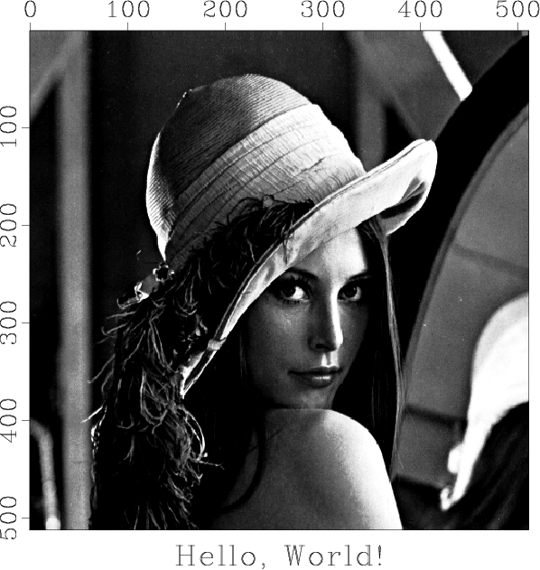
Fig directory and displayed on the screen. The output should
look like Figure 2.
|
lena
Figure 2. The output of the first numerical experiment. |
|
|---|---|
|
|
Ready to experiment? Try some of the following:
bash$ scons -c -Q
Removed lena.img
Removed lena.hdr
Removed lena.rsf
Removed /datapath/lena.rsf@
Removed Fig/lena.vpl
Run scons again, and the default target will be regenerated.
bash$ scons -Q
retrieve(["lena.img"], [])
echo n1=512 n2=513 in=lena.img data_format=native_uchar > lena.hdr
< lena.hdr /RSF/bin/sfdd type=float | /RSF/bin/sfwindow f2=1 > lena.rsf
< lena.rsf /RSF/bin/sfgrey title="Hello, World!" transp=n color=b \
bias=128 clip=100 screenratio=1 > Fig/lena.vpl
bash$ scons -Q view
< lena.rsf /RSF/bin/sfgrey title="Hello, World!" transp=n color=b \
bias=128 clip=50 screenratio=1 > Fig/lena.vpl
/RSF/bin/xtpen Fig/lena.vpl
SCons is smart enough to recognize that your editing did not affect any of the previous results in the data flow chain! Keeping track of dependencies is the main feature that separates data processing and computational experimenting with SCons from using linear shell scripts. For computationally demanding data processing, this feature can save you a lot of time and can make your experiments more interactive and enjoyable.
The summary of our SCons commands is given in Table 2.
| scons |
| Generate |
| scons |
| Generate default targets (usually figures specified in Result.) |
| scons view or scons |
| Generate Result figures and display them on the screen. |
| scons print or scons |
| Generate Result figures and print them. |
| scons lock or scons |
| Generate Result figures and install them in a separate location. |
| scons test or scons |
| Generate Result figures and compare them with the corresponding ``locked'' figures stored in a separate location (regression testing). |
| scons |
| Generate the |
| scons TIMER=y ... |
| Time the execution of each step in the processing flow (using the Unix time utility.) |
| scons CHECKPAR=y ... |
| Check the names and values of all parameters supplied to Madagascar modules in the processing flows before executing anything (guards against incorrect input.) This option is new and experimental. |
|
|
|
|
Reproducible computational experiments using SCons |