|
|
|
|
Madagascar tutorial |

|
|---|
|
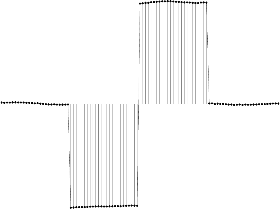
step,smooth
Figure 3. (a) 1-D synthetic to test edge-preserving smoothing. (b) Output of conventional triangle smoothing. |
|
|
To better understand the effect of smoothing, you decide to create a one-dimensional synthetic example shown in Figure 3(a). The synthetic contains both sharp edges and random noise. The output of conventional triangle smoothing is shown in Figure 3(b). We see an effect similar to the one in the real data example: random noise gets removed by smoothing at the expense of blurring the edges. Can you do better?


|
|---|
|
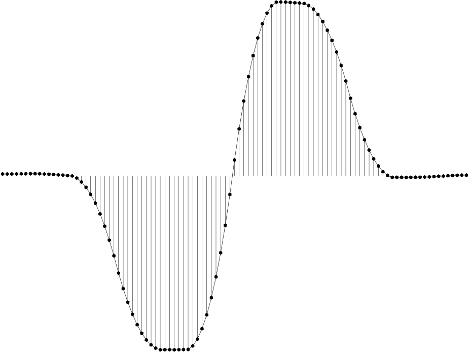
spray,local
Figure 4. (a) Input synthetic trace duplicated multiple times. (b) Duplicated traces shifted so that each data sample gets surrounded by its neighbors. The original trace is in the middle. |
|
|
To better understand what is happening in the process of smoothing, let us convert 1-D signal into a 2-D signal by first replicating the trace several times and then shifting the replicated traces with respect to the original trace (Figure 4). This creates a 2-D dataset, where each sample on the original trace is surrounded by samples from neighboring traces.
Every local filtering operation can be understood as stacking traces from Figure 4(b) multiplied by weights that correspond to the filter coefficients.
bash$ cd ../local
bash$ scons smooth.view smooth2.viewOpen the SConstruct file in a text editor to verify that the first image is computed by sfsmooth and the second image is computed by applying triangle weights and stacking. To compare the two images by flipping between them, run
bash$ sfpen Fig/smooth.vpl Fig/smooth2.vpl
bash$ scons triangle.view similarity.viewThe results should look similar to Figure 5.

|
|---|
|
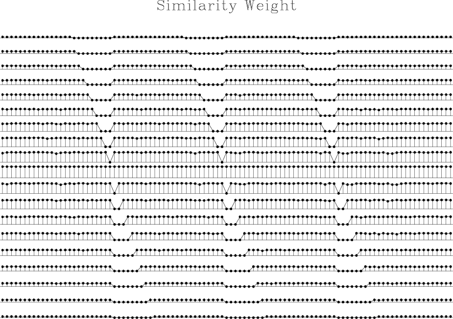
triangle,similarity
Figure 5. (a) Linear and stationary triangle weights. (b) Non-linear and non-stationary weights reflecting both distance between data points and similarity in data values. |
|
|
|
nlsmooth
Figure 6. Output of non-local smoothing |
|
|---|---|
|
|
Figure 6 shows that non-linear filtering can eliminate random noise while preserving the edges. The problem is solved! Now let us apply the result to our original problem.
|
|
|
|
Madagascar tutorial |