Wavefield Seismic Imaging tutorial: ``exploding reflector'' modeling/migration

Example

I illustrate the zero-offset modelind and migration methodology using the Sigsbee 2A synthetic model. This model is based on the Sigsbee structure in the Gulf of Mexico and the velocity is illustrated in Figure 2. The model is characterized by a massive salt body close to the water bottom and surrounded by sediments. The salt velocity is $4.5$  km/s and the surrounding sediment velocities range from approximately $1.5$ to $3.25$  km/s.

vstr
Figure 1. Stratigraphic Sigsbee 2A velocity model.

In this experiment, I consider sources distributed uniformly in the subsalt region of the model. The data are acquired in a borehole array, located at $x=8.5$  km and in a horizontal array located at $z=1.5$  km. In order to avoid multiple scattering in the subsurface, I simulate waves with a smooth version of the Sigsbee model, illustrated in Figure 3, and with constant density.

vsmo
Figure 2. Smooth Sigsbee 2A velocity model.

Using the MADAGASCAR program sfawefd2d, we can simulate wavefields from the distributed sources. Figures 4a-4h show wavefield snapshots in order of increasing times. We can observe waves propagating from all subsalt sources, interacting with the variable velocity medium and arriving at the vertical and horizontal arrays.

2wfld-01,wfld-03,wfld-05,wfld-07,wfld-09,wfld-11,wfld-13,wfld-15 width=0.45Wavefield snapshots at increasing times.

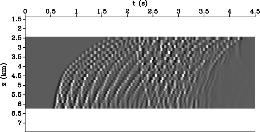
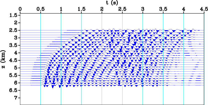
Figures 5a and 5b show the data observed at the horizontal array in variable density and wiggle plotting formats, respectively. Similarly, Figures 6a and 6b show the data observed in the vertical array using the same plotting formats. The data are just subsets of the same wavefields at the respective receiver positions and capture the complications observed in the wavefield, i.e. triplications due to lateral velocity variation.

datH,wigH
Figure 3. Acoustic data observed in the horizontal array.

datV,wigV
Figure 4. Acoustic data observed in the vertical array.

In zero-offset migration, we backprogate the acoustic wavefields using the acquired data as boundary conditions. The image is the wavefield at time zero. Since we can acquire data at different locations in space, the reconstructed wavefields depend on the acquisition geometry, thus limiting the illumination in the subsurface. Therefore, the migrated images depend on the acquisition array, as illustrated in Figures 7a and 7b for the horizontal and vertical arrays, respectively. We can also obtain images by migrating the data observed in both the horizontal and vertical arrays, as illustrated in Figure 8, thus increasing the acquisition aperture and the subsurface illumination.

imgH,imgV
Figure 5. Migrated images for data acquired in (a) the horizontal array and (b) the vertical array.

imgA
Figure 6. Migrated image for data acquired in both the horizontal and vertical arrays.

Wavefield Seismic Imaging tutorial: ``exploding reflector'' modeling/migration