|
|
|
|
Time-lapse image registration using the local similarity attribute |
|
|---|
|
modl,rat
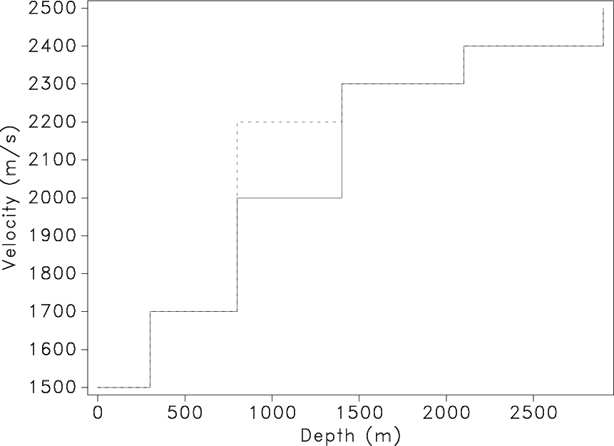
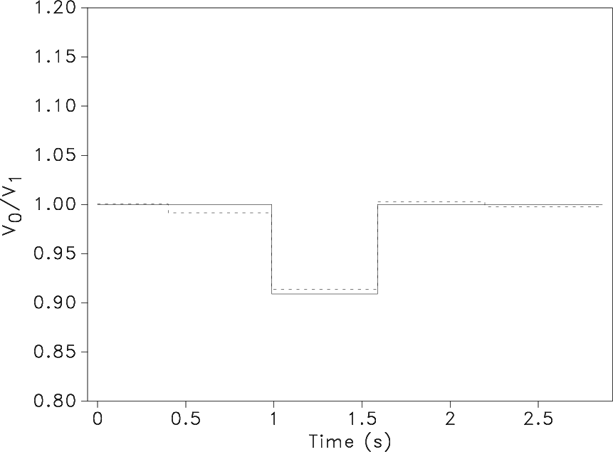
Figure 1. (a) 1-D synthetic velocity model before (solid line) and after (dashed line) reservoir production. (b) True (solid line) and estimated (dashed line) interval velocity ratio. |
|
|
|
|---|
|
data,warp
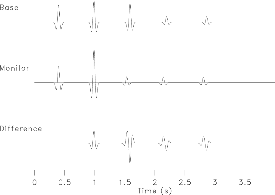
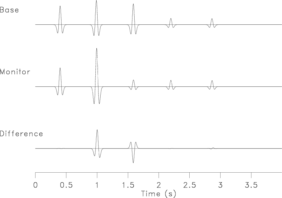
Figure 2. 1-D synthetic seismic images and the time-lapse difference initially (a) and after image registration (b). |
|
|
|
|---|
|
scan100
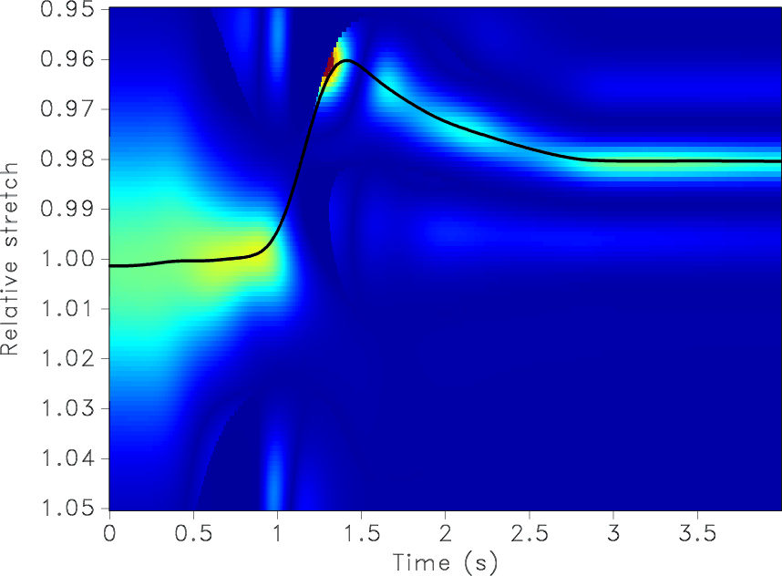
Figure 3. (a) Local similarity scan for detecting the warping function in the 1-D synthetic model. Red colors indicate large similarity. The black curve shows an automatically detected trend. |
|
|
Figure 1(a) shows a simplistic five-layer velocity model,
where we introduce a velocity increase in one of the layers to
simulate a time-lapse effect. After generating synthetic image
traces, we can observe, in Figure 2(a), that the time-lapse
difference contains changes not only at the reservoir itself but also
at interfaces below the reservoir. Additionally, the image amplitude
and the wavelet shape at the reservoir bottom are incorrect. These
artifact differences are caused by time shifts resulting from the
velocity change. After detecting the warping function ![]() from the
local similarity scan, shown in Figure 3, and
applying it to the time-lapse image, the difference correctly
identifies changes in reflectivity only at the top and the bottom of
the producing reservoir [Figure 2(b)]. To implement the
local similarity scan, we use the relative stretch measure
from the
local similarity scan, shown in Figure 3, and
applying it to the time-lapse image, the difference correctly
identifies changes in reflectivity only at the top and the bottom of
the producing reservoir [Figure 2(b)]. To implement the
local similarity scan, we use the relative stretch measure
![]() . When the two images are perfectly aligned,
. When the two images are perfectly aligned,
![]() . Deviations of
. Deviations of ![]() from one indicate possible
misalignment. Finally, we apply equation 9 to estimate
interval velocity changes in the reservoir and observe a reasonably
good match with the exact synthetic model [Figure 1(b)].
from one indicate possible
misalignment. Finally, we apply equation 9 to estimate
interval velocity changes in the reservoir and observe a reasonably
good match with the exact synthetic model [Figure 1(b)].
|
|
|
|
Time-lapse image registration using the local similarity attribute |