|
|
|
|
Nonlinear structure-enhancing filtering using plane-wave prediction |
The method of plane-wave destruction (Claerbout, 1992) uses a local
plane-wave model for characterizing the structure of seismic data. It
finds numerous applications in seismic imaging and data processing
(Fomel, 2002). Letting a seismic section, ![]() , be a
collection of traces,
, be a
collection of traces,
![]() , the plane-wave destruction
operation can be defined in a linear operator notation as
, the plane-wave destruction
operation can be defined in a linear operator notation as
where ![]() is the destruction residual and
is the destruction residual and ![]() is the
nonstationary plane-wave destruction operator defined as follows
is the
nonstationary plane-wave destruction operator defined as follows
The least-squares minimization of ![]() is achieved by using
iterative conjugate-gradient (CG) method and smooth
regularization. Local dip at a fault position cannot be accurately
estimated, its value will depend on the initial slope estimate and
regularization.
is achieved by using
iterative conjugate-gradient (CG) method and smooth
regularization. Local dip at a fault position cannot be accurately
estimated, its value will depend on the initial slope estimate and
regularization.
Prediction of a trace from a distant neighbor can be
accomplished by simple recursion, i.e., predicting trace ![]() from
trace
from
trace ![]() is simply
is simply
Fomel (2008) applied plane-wave prediction to predictive painting of seismic images. In this paper, we use a similar construction to recursively predict a trace from its neighbors.
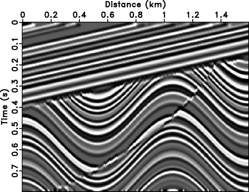
An example is shown in Figure 1a.
The input data is borrowed from Claerbout (2008): a synthetic
seismic image containing dipping beds, an uncomformity, and a
fault. Figure 1b shows the same
image with Gaussian noise
added. Figure 1c shows local
slopes measured from the noisy image by plane-wave destruction. The
estimated slope field correctly depicts the constant slope in the top
part of the image and the sinusoidal variation of slopes in the
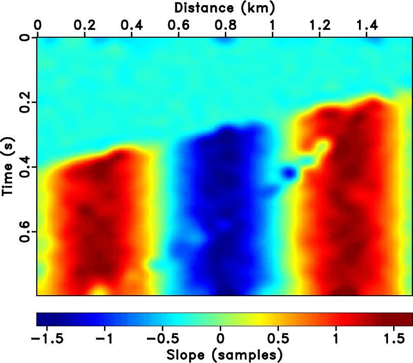
bottom. In the next step, we predict every trace from its neighbor
traces according to the local slope, as described by
Fomel (2008). We chose a total of 14 prediction steps (7 from the
left and 7 from the right), which, with the addition of the original
section, generated a data volume
(Figure 1d). The prediction
axis corresponds to index ![]() in equation 3. The volume
is flat along the prediction direction, which confirms the ability of
plane-wave destruction to follow the local
structure. However, it still contains some discontinuous information
because of the faults. In the next step, we apply nonlinear
structure-enhancing filtering to process the data along the prediction
direction.
in equation 3. The volume
is flat along the prediction direction, which confirms the ability of
plane-wave destruction to follow the local
structure. However, it still contains some discontinuous information
because of the faults. In the next step, we apply nonlinear
structure-enhancing filtering to process the data along the prediction
direction.

|
|---|
|
sigmoid1,gnoise1,ndip1,cube
Figure 1. Noise-free synthetic image (a), noisy image (b), local slopes estimated from Figure 1b (c), and predictive data volume, where every trace is supplemented with predictions from its neighbors (d). |
|
|
|
|
|
|
Nonlinear structure-enhancing filtering using plane-wave prediction |

![\begin{displaymath}
\left[\begin{array}{c}
\mathbf{d}_1 \\
\mathbf{d}_2 \\...
...{s}_3 \\
\cdots \\
\mathbf{s}_N \\
\end{array}\right]\;,
\end{displaymath}](img15.png)