 |
 |
 |
 | Stacking seismic data using local correlation |  |
![[pdf]](icons/pdf.png) |
Next: Stacking using local correlation
Up: Methodology
Previous: Methodology
The global uncentered correlation coefficient between two discrete
signals  and
and  can be defined as the functional
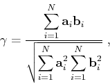 |
(1) |
where N is the length of a signal. The global correlation in equation 1
supplies only one number for the whole signal. For measuring the
similarity between two signals locally, one can define the sliding-window
correlation coefficient
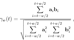 |
(2) |
where  is window length.
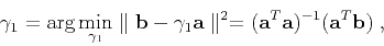
Fomel (2007a) proposes the local correlation attribute that identifies
local changes in signal similarity in a more elegant way. In a linear
algebra notation, the correlation coefficient in equation 1 can be
represented as a product of two least-squares inverses  and
and  :
:
 |
(3) |
 |
(4) |
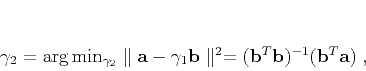 |
(5) |
where  and
and  are vector notions for and
. Let
are vector notions for and
. Let  and
and  be two diagonal
operators composed of the elements of a and b. Localizing
equations 4 and 5 amounts to adding regularization to
inversion. Using shaping regularization (Fomel, 2007b), scalars
and turn into vectors
be two diagonal
operators composed of the elements of a and b. Localizing
equations 4 and 5 amounts to adding regularization to
inversion. Using shaping regularization (Fomel, 2007b), scalars
and turn into vectors  and
and  , defined as
![\begin{displaymath}
\mathbf{c}_1 = [\lambda^2 \mathbf{I} + \mathbf{S}(\mathbf{A...
...mbda^2 \mathbf{I})]^{-1}\mathbf{S}\mathbf{A}^T\mathbf{b}\;,
\end{displaymath}](img25.png) |
(6) |
![\begin{displaymath}
\mathbf{c}_2 = [\lambda^2 \mathbf{I} + \mathbf{S}(\mathbf{B...
...mbda^2 \mathbf{I})]^{-1}\mathbf{S}\mathbf{B}^T\mathbf{a}\;,
\end{displaymath}](img26.png) |
(7) |
where  scaling controls relative scaling of operators
and and
where
scaling controls relative scaling of operators
and and
where  is a shaping operator such as Gaussian smoothing with an
adjustable radius. The component-wise product of vectors and
defines the local correlation measure. Local correlation is a measure
of the similarity between two signals.
An iterative, conjugate-gradient inversion for computing the inverse
operators can be applied in equations 6 and 7.
Interestingly, the output of the first iteration is equivalent to the
algorithm of fast local
cross-correlation proposed by Hale (2006).
is a shaping operator such as Gaussian smoothing with an
adjustable radius. The component-wise product of vectors and
defines the local correlation measure. Local correlation is a measure
of the similarity between two signals.
An iterative, conjugate-gradient inversion for computing the inverse
operators can be applied in equations 6 and 7.
Interestingly, the output of the first iteration is equivalent to the
algorithm of fast local
cross-correlation proposed by Hale (2006).
|
|
|
|
| Stacking seismic data using local correlation | |
|
Next: Stacking using local correlation
Up: Methodology
Previous: Methodology
2013-03-02