|
|
|
|
Shaping regularization in geophysical estimation problems |
|
|---|
|
bei-fmg2
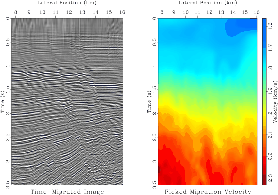
Figure 8. Left: time-migrated image. Right: The corresponding migration velocity from automatic picking. |
|
|
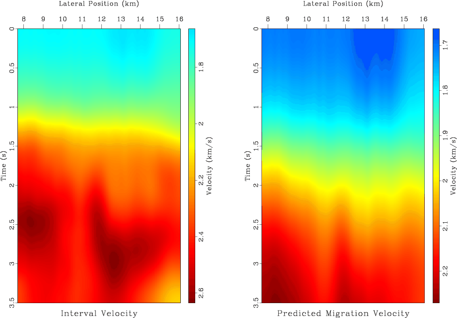
The task of this example is to convert the time migration velocity to
the interval velocity. I use the simple approach of Dix inversion
(Dix, 1955) formulated as a regularized inverse problem
(Valenciano et al., 2004). In this case, the forward operator ![]() in
equation 11 is a weighted time
integration. There is a choice in choosing the shaping
operator
in
equation 11 is a weighted time
integration. There is a choice in choosing the shaping
operator ![]() .
.
Figure 9 shows the result of inversion with shaping by triangle smoothing. While the interval velocity model yields a good prediction of the measured velocity, it may not appear geologically plausible because the velocity structure does not follow the structure of seismic reflectors as seen in the migrated image.
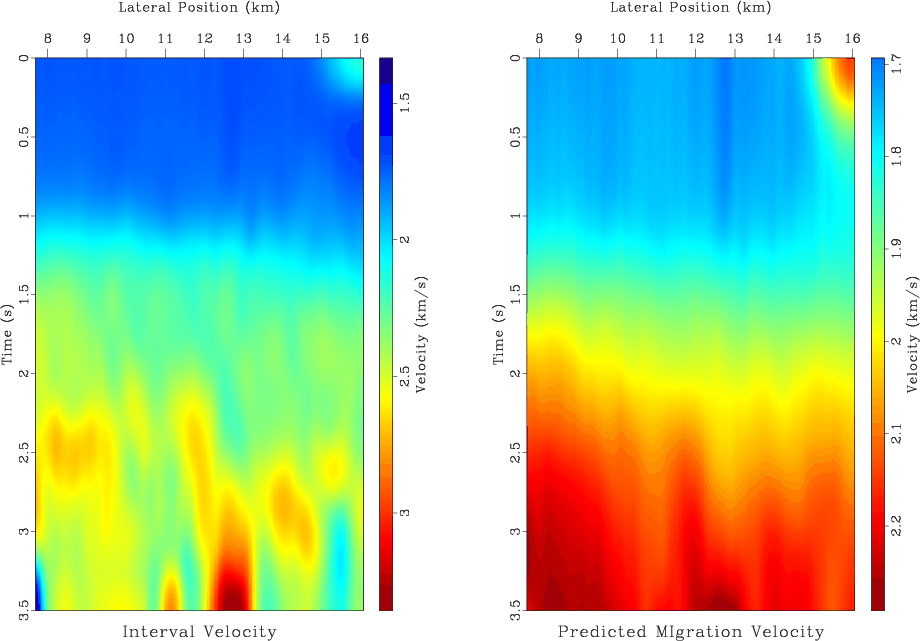
Following the ideas of steering filters (Clapp et al., 1998,2004)
and plane-wave construction (Fomel and Guitton, 2006), I estimate local slopes in
the migration image using the method of plane-wave destruction
(Fomel, 2002) and define a triangle plane-wave shaping
operator ![]() using the method of the previous
section. The result of inversion, shown in Figures 10
and 11, makes the estimated interval velocity follow
the geological structure and thus appear more plausible for
direct interpretation. Similar results were obtained by Fomel and Guitton (2006)
using model parameterization by plane-wave construction but at a
higher computational cost. In the case of shaping regularization,
about 25 efficient iterations were sufficient to converge to the
machine precision accuracy.
using the method of the previous
section. The result of inversion, shown in Figures 10
and 11, makes the estimated interval velocity follow
the geological structure and thus appear more plausible for
direct interpretation. Similar results were obtained by Fomel and Guitton (2006)
using model parameterization by plane-wave construction but at a
higher computational cost. In the case of shaping regularization,
about 25 efficient iterations were sufficient to converge to the
machine precision accuracy.
|
|---|
|
bei-dix
Figure 9. Left: estimated interval velocity. Right: predicted migration velocity. Shaping by triangle smoothing. |
|
|
|
|---|
|
bei-shp
Figure 10. Left: estimated interval velocity. Right: predicted migration velocity. Shaping by triangle local plane-wave smoothing creates a velocity model consistent with the reflector structure. |
|
|
|
|---|
|
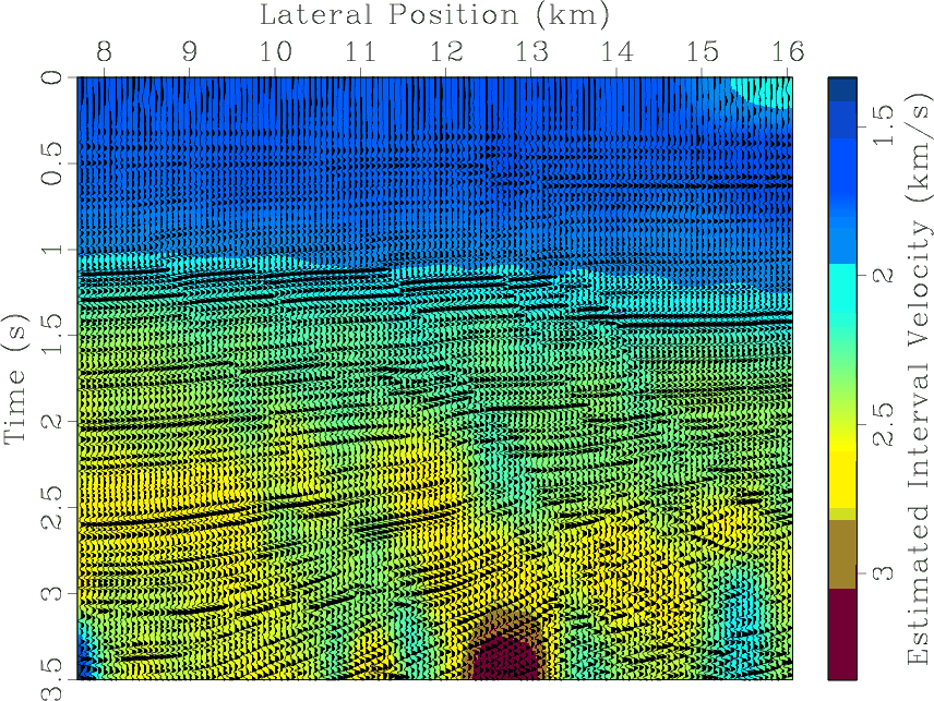
bei-shpw
Figure 11. Seismic image from Figure 8 overlaid on top of the interval velocity model estimated with triangle plane-wave shaping regularization. |
|
|
|
|
|
|
Shaping regularization in geophysical estimation problems |