|
|
|
|
Seislet transform and seislet frame |
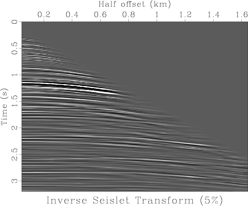
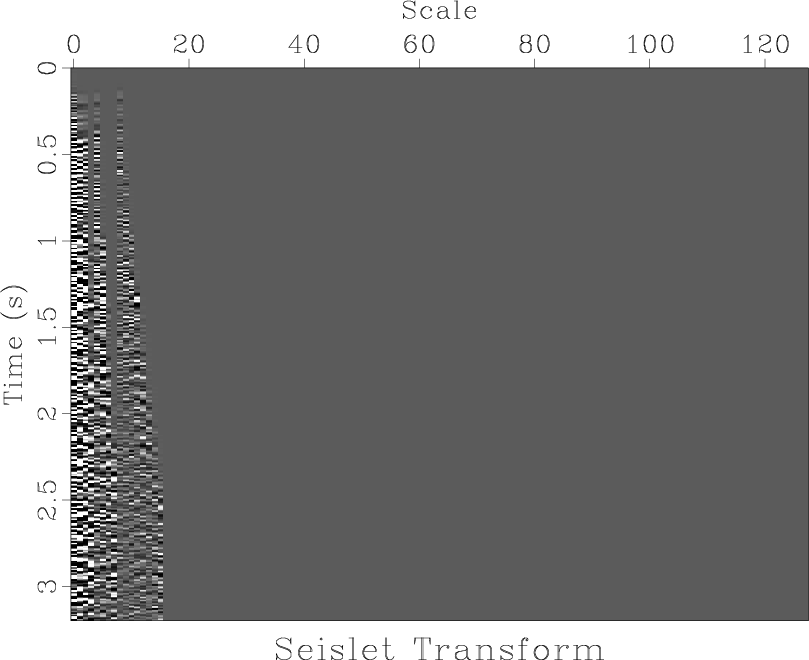
Figure 7(a) shows a common-midpoint gather from a North Sea dataset. Plane-wave destruction estimates local slopes shown in Figure 7(b) and enables the 2-D seislet transform shown in Figure 8(a). Small dynamic range of seislet coefficients implies a good compression ratio. Figure 8(b) shows data reconstruction using only 5% of the significant seislet coefficients.
If we choose the significant coefficients at the coarse scale and zero out difference coefficients at the finer scales, the inverse transform will effectively remove incoherent noise from the gather (Figure 8). Thus, denoising is a naturally defined operation in the 2-D seislet domain (Figure 9).
If we extend the seislet transform domain and interpolate the smooth local slope to a finer grid, the inverse seislet transform will accomplish trace interpolation of the input gather (Figure 10). We extend not simply with zeros but with small random noise to account for the fact that realistic noise is unpredictable and therefore exists on different scale levels. In this example, the number of traces is increased by four. Thus, trace interpolation also turns out to be a natural operation when viewed from the 2-D seislet domain.


|
|---|
|
gath,gathdip
Figure 7. Common-midpoint gather (a) and local slopes estimated by plane-wave destruction (b). |
|
|

|
|---|
|
gathseis,gathsrec5
Figure 8. Seislet transform of the input gather (a) and (a) and data reconstruction using only 5% of significant seislet coefficients (b). |
|
|

|
|---|
|
sign,gathslet16
Figure 9. Zeroing seislet difference coefficients at fine scales (a) enables effective denoising of the reconstructed data (b). |
|
|


|
|---|
|
seis4,gath4
Figure 10. Extending seislet transform with random noise (a) enables trace interpolation in the reconstructed data. The interpolated section (b) has 4 times more traces than the original shown in Figure 7(a). |
|
|
|
|
|
|
Seislet transform and seislet frame |