 |
 |
 |
 | Seislet transform and seislet frame |  |
![[pdf]](icons/pdf.png) |
Next: 2-D seislet transform
Up: From wavelets to seislets
Previous: From wavelets to seislets
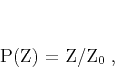
The prediction and update operators employed in the lifting scheme can
be understood as digital filters. In the  -transform notation, the
Haar prediction filter from equation 3 is
-transform notation, the
Haar prediction filter from equation 3 is
 |
(8) |
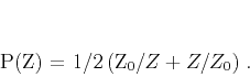
(shifting each sample by one), and the linear interpolation filter
from equation 4 is
 |
(9) |
These predictions are appropriate for smooth signals but may not be
optimal for a sinusoidal signal. In
comparison, the prediction
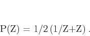
 |
(10) |
where
 , perfectly characterizes a
sinusoid with
, perfectly characterizes a
sinusoid with  circular frequency sampled on a
  grid. In other words, if a constant signal (
 ) is perfectly
predicted by shifting each trace to its neighbor, a sinusoidal signal
(
) is perfectly
predicted by shifting each trace to its neighbor, a sinusoidal signal
( ) requires the shift to be modulated by an appropriate
frequency.
Likewise, the linear interpolation in equation 9 needs to be
replaced by a filter tuned to a particular frequency in order to
predict a sinusoidal signal with that frequency perfectly:
) requires the shift to be modulated by an appropriate
frequency.
Likewise, the linear interpolation in equation 9 needs to be
replaced by a filter tuned to a particular frequency in order to
predict a sinusoidal signal with that frequency perfectly:
 |
(11) |
The analysis easily extends to higher-order filters.
|
|
|
|
| Seislet transform and seislet frame | |
|
Next: 2-D seislet transform
Up: From wavelets to seislets
Previous: From wavelets to seislets
2013-03-02