 |
 |
 |
 | Seislet transform and seislet frame |  |
![[pdf]](icons/pdf.png) |
Next: Bibliography
Up: Fomel and Liu: Seislet
Previous: Conclusions
We thank BGP Americas for a partial financial support of this work. The first
author is grateful to Huub Douma for inspiring discussions and for suggesting
the name ``seislet''. This publication is authorized by the Director, Bureau
of Economic Geology, The University of Texas at Austin.
Appendix
A
Review of plane-wave destruction
This appendix reviews the basic theory of plane-wave destruction
(Fomel, 2002).
Following the physical model of local plane waves, we
define the mathematical basis of plane-wave destruction filters via
the local plane differential equation (Claerbout, 1992)
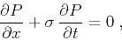 |
(19) |
where  is the wave field, and
  is the local slope, which may
also depend on
is the local slope, which may
also depend on  and
and  . In the case of a constant slope,
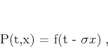
equation A-1 has the simple general solution
. In the case of a constant slope,
equation A-1 has the simple general solution
 |
(20) |
where  is an arbitrary waveform. Equation A-2 is
nothing more than a mathematical description of a plane wave.
is an arbitrary waveform. Equation A-2 is
nothing more than a mathematical description of a plane wave.
If we assume that the slope does not depend on , we can
transform equation A-1 to the frequency domain, where it
takes the form of the ordinary differential equation
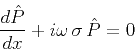 |
(21) |
and has the general solution
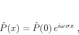 |
(22) |
where  is the Fourier transform of
  . The complex
exponential term in equation A-4 simply represents a shift
of a -trace according to the slope and the trace separation
.
. The complex
exponential term in equation A-4 simply represents a shift
of a -trace according to the slope and the trace separation
.
In the frequency domain, the operator for transforming the trace  to the neighboring trace is a multiplication by
 . In other words, a plane wave can be perfectly
predicted by a two-term prediction-error filter in the
. In other words, a plane wave can be perfectly
predicted by a two-term prediction-error filter in the  -
- domain:
 |
(23) |
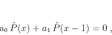
where  and
and
 . The goal of
predicting several plane waves can be accomplished by cascading
several two-term filters. In fact, any - prediction-error
filter represented in the
. The goal of
predicting several plane waves can be accomplished by cascading
several two-term filters. In fact, any - prediction-error
filter represented in the  -transform notation as
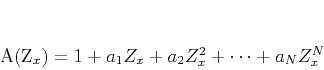 |
(24) |
can be factored into a product of two-term filters:
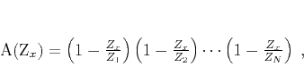 |
(25) |
where
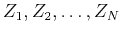 are the zeroes of
polynomial A-6. According to equation A-5,
the phase of each zero corresponds to the slope of a local plane wave
multiplied by the frequency. Zeroes that are not on the unit circle
carry an additional amplitude gain not included in
equation A-3.
are the zeroes of
polynomial A-6. According to equation A-5,
the phase of each zero corresponds to the slope of a local plane wave
multiplied by the frequency. Zeroes that are not on the unit circle
carry an additional amplitude gain not included in
equation A-3.
In order to incorporate time-varying slopes, we need to return to
the time domain and look for an appropriate analog of the phase-shift
operator A-4 and the plane-prediction
filter A-5. An important property of plane-wave
propagation across different traces is that the total energy of the
propagating wave stays invariant throughout the process: the energy of
the wave at one trace is completely transmitted to the next trace.
This property
is assured in the frequency-domain solution A-4 by the fact
that the spectrum of the complex exponential
is
equal to one. In the time domain, we can reach an equivalent effect
by using an all-pass digital filter. In the -transform notation,
convolution with an all-pass filter takes the form
 |
(26) |
where
 denotes the -transform of the corresponding
trace, and the ratio
denotes the -transform of the corresponding
trace, and the ratio
 is an all-pass digital filter
approximating the time-shift operator
is an all-pass digital filter
approximating the time-shift operator
 . In
finite-difference terms, equation A-8 represents an
implicit finite-difference scheme for solving equation A-1
with the initial conditions at a constant . The coefficients of
filter
. In
finite-difference terms, equation A-8 represents an
implicit finite-difference scheme for solving equation A-1
with the initial conditions at a constant . The coefficients of
filter  can be determined, for example, by fitting the filter
frequency response at low frequencies to the response of the
phase-shift operator. This leads to a version of Thiran's
maximally-flat all-pass fractional-delay filters (Välimäki and Laakso, 2001; Thiran, 1971).
can be determined, for example, by fitting the filter
frequency response at low frequencies to the response of the
phase-shift operator. This leads to a version of Thiran's
maximally-flat all-pass fractional-delay filters (Välimäki and Laakso, 2001; Thiran, 1971).
Taking both dimensions into consideration,
equation A-8 transforms to the prediction equation
analogous to A-5 with the 2-D prediction filter
 |
(27) |
In order to characterize several plane waves, we can cascade several
filters of the form A-9 in a manner similar to that of
equation A-7. A modified version of the filter
 , namely the filter
 |
(28) |
avoids the need for polynomial division. In case of a
3-point filter , the 2-D filter A-10 has exactly
six coefficients. It consists of two columns, each column having three
coefficients and the second column being a reversed copy of the first
one.
|
|
|
|
| Seislet transform and seislet frame | |
|
Next: Bibliography
Up: Fomel and Liu: Seislet
Previous: Conclusions
2013-03-02