A reversible transform for seismic data processing

Conclusions

Using the theory of nonstationary filtering, we have developed a general transform that applies and removes many common seismic data processing and imaging operations. Any data processing or imaging step that can be viewed as a nonstationary shift in any domain is a special case of this transform. We have provided a derivation of the general data processing transform and we have used NMO as a familiar example.

Like the Fourier transform, the data processing transform is a mixed-domain transform. In the general case, the input data should be viewed as an image, and then a distorted version of that image is the desired output. The data processing transform moves data directly between the Fourier spectrum of the input image and the corrected image. Regardless of the physical meaning of input and the Fourier coordinates, viewing the input and output data each as an image makes the general application of the transform to any processing step clear. The physical meaning of the transform coordinates and distortions can be defined only when discussing specific processing steps.

Common nonstationary shifts in seismic data processing are often nonphysical, as they do not conserve the energy of a given input signal. The general data processing transform predicts and quantifies the change in energy caused by such processing steps. Processing artifacts such as NMO stretch associated with the NMO correction and Stolt stretch associated with Stolt and frequency-wavenumber migration are examples of this type of nonphysical energy change. Under the framework of the general data processing transform, these effects are both special cases of, and are easily quantified by, the nonstationary scaling function $\alpha (q)$ . We have shown that the data processing transform is reversible by accounting for these energy changes while simultaneously reversing the kinematic shift applied by the forward transform.

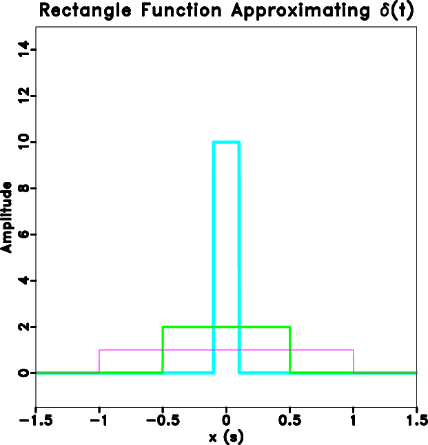
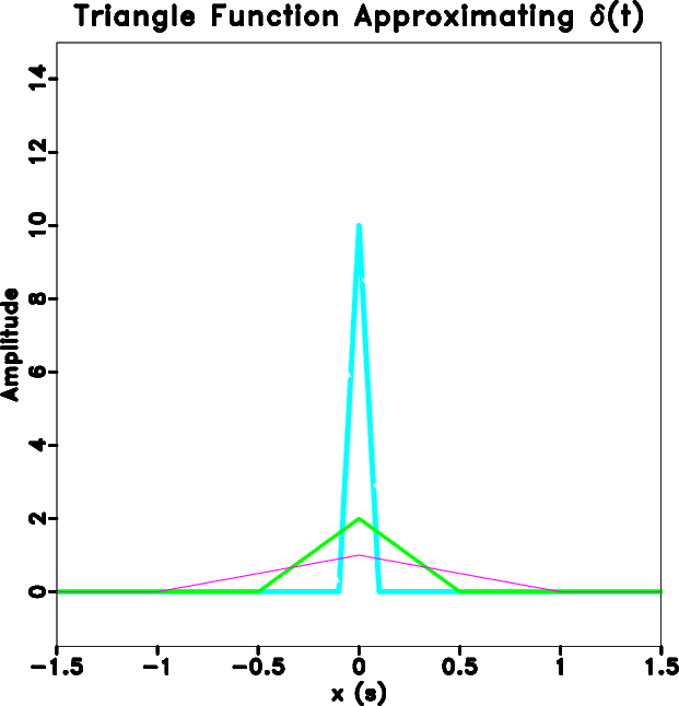
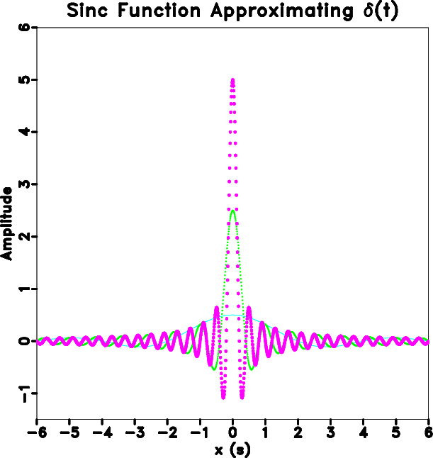
Rather than explicitly interpolating discrete data, the data processing transform assumes that the input signal behaves according to the Fourier basis between samples. The Fourier transform itself predicts a continuous form of given discrete data, and the transform here performs a nonstationary shift on this continuous function. Just as in the stationary case, nonstationary shifts can be viewed as convolution with a Dirac delta function. We have demonstrated how common interpolants such as boxcar, triangle, and sinc functions approximate the delta function, but add assumptions about how the input signal behaves in between samples which may contradict the Fourier basis. By analysis in both input and Fourier domains, we have shown that the use of an untruncated sinc function as an interpolant is equivalent to the discrete form of this transform.

Having a reversible transform for seismic data processing allows the various stages of a processing flow to be viewed as valid processing domains. For example, one may use this transform to apply a correction to the input data which organizes it into a format better suited for multiple attenuation, then perform multiple attenuation, and last transform back to the input domain with no residual effects of the correction itself. Further, the discrete form of this general transform provides a straightforward framework for constructing and understanding the matrix operators associated with seismic imaging steps. Future studies may be able to exploit symmetries of these operators to improve computational efficiency while mitigating interpolation artifacts. We anticipate a variety of future applications of the reversible transform using these concepts.

nearest Figure 7. Nearest-neighbour interpolant approaching $\delta \left ( t \right )$ . As $\epsilon$ approaches zero, the rectangle function defined by equation 28 approaches the Dirac delta function. Thin magenta line: $\epsilon =1.0$ . Green line: $\epsilon =0.5$ . Thick cyan line: $\epsilon =0.1$ .

linear Figure 8. Linear interpolant approaching $\delta \left ( t \right )$ . As $\epsilon$ approaches zero, the triangle function defined by equation 30 approaches the Dirac delta function. Thin magenta line: $\epsilon =1.0$ . Green line: $\epsilon =0.5$ . Thick cyan line: $\epsilon =0.1$ .

sinc Figure 9. Sinc interpolant approaching $\delta \left ( t \right )$ . As $\epsilon$ approaches infinity, the sinc-function defined by equation 32 approaches the Dirac delta function. Magenta * line: $\epsilon =5.0$ , Dotted green line: $\epsilon =2.5$ . Solid cyan line: $\epsilon =0.5$ .

A reversible transform for seismic data processing