Velocity-independent time-domain seismic imaging using local event slopes

Normal moveout

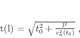
Let us consider the classic hyperbolic model of reflection moveout:

$$t(l) = \sqrt{t_0^2 + \frac{l^2}{v_n^2(t_0)}}\;,$$ (1)

where $t_0$ is the zero-offset traveltime, $t(l)$ is the corresponding traveltime recorded at offset $l$, and $v_n(t_0)$ is the stacking or RMS velocity. As follows from equation 1, the traveltime slope $p= d t/d l$ is given by

$${p} = {\frac{l}{t\,v_n^2(t_0)}}\;.$$ (2)

Knowing the local slope $p(t,l)$ in a common-midpoint gather, one can effectively eliminate the velocity $v(t_0)$ from equations 1 and 2 arriving at the velocity-independent moveout equation (Ottolini, 1983)

$$t_0 = \sqrt{t^2 - t\,p(t,l)\,l}\;.$$ (3)

Equation 3 describes a direct mapping from prestack data to the zero-offset time. This equation constitutes an oriented normal moveout correction. As follows from equation 2, the velocity is mapped as follows:

$${\frac{1}{v_n^2}} = p(t,l)\,{\frac{t}{l}}\;.$$ (4)

Unlike its role in the conventional normal moveout (NMO), velocity is not a requirement for the moveout correction but rather a data attribute derived from the local slopes and mappable directly to the appropriate zero-offset time.

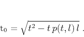
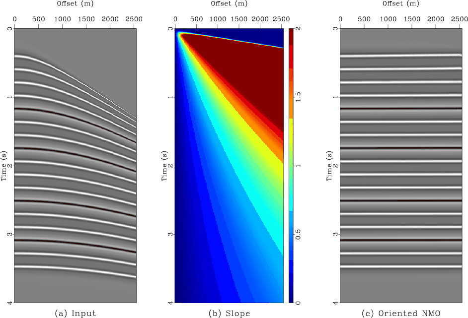
A simple synthetic example is shown in Figure 1. The synthetic data (Figure 1a) were generated by applying inverse NMO with time-variable velocity and represent perfectly hyperbolic events. Figure 1b shows local event slopes measured from the data using the plane-wave destruction algorithm of Fomel (2002). Plane-wave destruction (Claerbout, 1992) works by making a prediction of each seismic trace from the neighboring trace along local slopes and then minimizing the prediction error by an iterative regularized least-squares optimization. Regularization controls smoothness of the estimated slope field. In this work, I use shaping regularization (Fomel, 2007) for an optimal smoothness control. Figure 1c shows the output of oriented NMO using equation 3. As expected, all events are perfectly flattened after NMO.

synt
Figure 1. a: A synthetic CMP gather composed of hyperbolas. b: Estimated local event slopes. c: The output of oriented velocity-independent NMO.

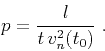
In conventional NMO processing, one scans a number of velocities, performs the corresponding number of moveout corrections, and picks the velocity trend from velocity spectra. In oriented processing, velocity becomes, according to equation 4, a data attribute rather than a prerequisite for imaging. Figure 2 shows a comparison between velocity spectra used for picking velocities in the conventional NMO processing and the velocity attribute mapped directly from the data space using equations 3 and 4. A noticeably higher resolution of the oriented map follows from the fact that only the true signal slopes are identified by the slope estimation algorithm. The slope uncertainty, unlike the velocity uncertainty, is not taken into account.

svsc
Figure 2. a: Velocity spectra using conventional velocity scanning. In the conventional NMO processing, the velocity trend is picked from velocity spectra prior to NMO. b: Velocity mapped from the data space using oriented NMO. The input for both plots is the synthetic CMP gather shown in Figure 1a. The red line indicates the exact velocity used for generating the synthetic data.

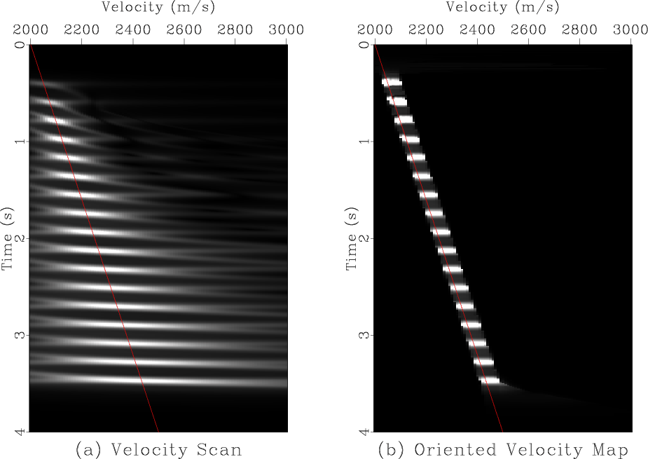
Figure 3 shows a field data example. The data are taken from a historic Gulf of Mexico dataset (Claerbout, 2005). Analogously to the synthetic case, a CMP gather (Figure 3a) is properly flattened (Figure 3c) by an application of oriented NMO using the local event slopes (Figure 3b) measured directly from the data. A comparison between conventional velocity spectra and the velocity mapping with oriented NMO is shown in Figure 4. Again, a significantly higher resolution is observed.

pnmo
Figure 3. a: A CMP gather from the Gulf of Mexico. b: estimated local event slopes. c: the output of oriented velocity-independent NMO.

bvsc
Figure 4. a: Velocity spectra using conventional velocity scanning. In the conventional NMO processing, the velocity trend is picked from velocity spectra prior to NMO. b: Velocity mapped from the data space using oriented NMO. The input for both plots is the CMP gather shown in Figure 3a. The red curve is an automatic pick of the velocity trend shown for comparison.

Velocity-independent time-domain seismic imaging using local event slopes