 |
 |
 |
 | Modeling of pseudo-acoustic P-waves in orthorhombic media with a lowrank approximation |  |
![[pdf]](icons/pdf.png) |
Next: Dispersion Relation for Orthorhombic
Up: Theory
Previous: Theory
The acoustic wave equation is widely used in
forward seismic modeling and reverse-time migration (Bednar, 2005; Etgen et al., 2009):
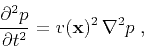 |
(1) |
where
 is the seismic pressure wavefield
and
is the seismic pressure wavefield
and  is the wave propagation velocity.
Assuming the model is homogeneous
 ,
after a Fourier transform in space,
we get the following explicit expression in the wavenumber domain:
,
after a Fourier transform in space,
we get the following explicit expression in the wavenumber domain:
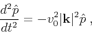 |
(2) |
where
 |
(3) |
Equation 2 has the following analytical solution:
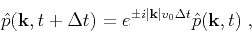 |
(4) |
which leads to
the well-known second-order time-marching scheme (Etgen, 1989; Soubaras and Zhang, 2008) :
 |
| |
|
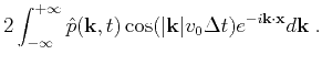 |
(5) |
Equation 5 provides a very accurate and efficient solution
in the case of a constant-velocity medium with the aid of FFTs.
When the seismic wave velocity varies in the medium,
equation 5 turns into a reasonable approximation by replacing  with , and taking small time steps,
  .
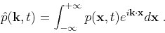
However, FFTs can no longer be applied directly to evaluate
the inverse Fourier transform,
because a space-wavenumber mixed-domain term appears in the integral operation:
.
However, FFTs can no longer be applied directly to evaluate
the inverse Fourier transform,
because a space-wavenumber mixed-domain term appears in the integral operation:
 |
(6) |
As a result, a straightforward numerical implementation of wave extrapolation
in a variable velocity medium with mixed-domain
matrix 6 will increase the cost from 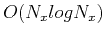 to
to  ,
the original cost for the homogeneous case,
in which
,
the original cost for the homogeneous case,
in which  is the total size of the three-dimensional space grid.
A number of numerical methods (Fomel et al., 2010; Du et al., 2010; Song et al., 2013,2011; Song and Fomel, 2011; Etgen and Brandsberg-Dahl, 2009; Liu et al., 2009; Zhang and Zhang, 2009; Fomel et al., 2012)
have been proposed to overcome this mixed-domain problem.
is the total size of the three-dimensional space grid.
A number of numerical methods (Fomel et al., 2010; Du et al., 2010; Song et al., 2013,2011; Song and Fomel, 2011; Etgen and Brandsberg-Dahl, 2009; Liu et al., 2009; Zhang and Zhang, 2009; Fomel et al., 2012)
have been proposed to overcome this mixed-domain problem.
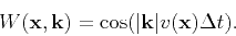
In the case of orthorhombic acoustic modeling,
we derive a new phase operator
 to replace
 of the isotropic model.
We describe the details in the next section.
of the isotropic model.
We describe the details in the next section.
|
|
|
|
| Modeling of pseudo-acoustic P-waves in orthorhombic media with a lowrank approximation | |
|
Next: Dispersion Relation for Orthorhombic
Up: Theory
Previous: Theory
2013-06-25