 |
 |
 |
 | OC-seislet: seislet transform construction with differential offset continuation |  |
![[pdf]](icons/pdf.png) |
Next: Bibliography
Up: Liu and Fomel: OC-seislet
Previous: Conclusions
We thank BGP Americas for a partial financial support of this
work. We thank Tamas Nemeth, Mauricio Sacchi, Sandra
Tegtmeier-Last, and two anonymous reviewers for their constructive
comments and suggestions. This publication was authorized by the
Director, Bureau of Economic Geology, The University of Texas at
Austin.
Appendix
A
Review of differential offset continuation
In this appendix, we review the theory of differential offset
continuation from Fomel (2003a,c). The partial
differential equation for offset continuation (differential azimuth
moveout) takes the form
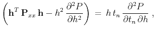 |
(13) |
where
 is the seismic data in the
midpoint-offset-time domain,
is the seismic data in the
midpoint-offset-time domain,  is the time coordinate after the
normal moveout (NMO) correction,
is the time coordinate after the
normal moveout (NMO) correction,
 denotes the transpose
of
denotes the transpose
of
 , and
, and
 is the tensor of the
second-order midpoint derivatives.
is the tensor of the
second-order midpoint derivatives.
A particularly efficient implementation of offset continuation results
from a log-stretch transform of the time coordinate
(Bolondi et al., 1982), followed by a Fourier transform of the stretched
time axis. After these transforms, the offset-continuation equation
takes the form
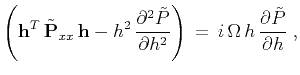 |
(14) |
where  is the dimensionless frequency corresponding to the
stretched time coordinate and
is the dimensionless frequency corresponding to the
stretched time coordinate and
 is the transformed data. As in other
frequency-space methods, equation A-2 can be applied
independently and in parallel on different frequency slices.
is the transformed data. As in other
frequency-space methods, equation A-2 can be applied
independently and in parallel on different frequency slices.
In the frequency-wavenumber domain, the extrapolation operator is
defined by solving an initial-value problem for
equation A-2. The analytical solution takes the form
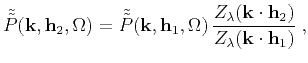 |
(15) |
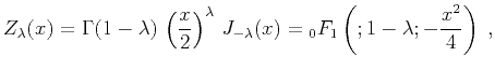
where
 is the double-Fourier-transformed
data,
is the double-Fourier-transformed
data,
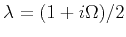 ,
,  is the special
function defined as
is the special
function defined as
 |
(16) |
 is the gamma function,
 is the Bessel function,
and
is the Bessel function,
and  is the confluent hypergeometric limit function (Petkovsek et al., 1996). The
wavenumber
is the confluent hypergeometric limit function (Petkovsek et al., 1996). The
wavenumber
 in equation A-3 corresponds to the
midpoint
in equation A-3 corresponds to the
midpoint
 in the original data domain. In high-frequency
asymptotics, the offset-continuation operator takes the form
in the original data domain. In high-frequency
asymptotics, the offset-continuation operator takes the form
![$\displaystyle \Tilde{\Tilde{P}}(\mathbf{k},\mathbf{h}_2,\Omega) \approx \Tilde{...
...ga\,\psi\left(\frac{2 \mathbf{k} \cdot \mathbf{h}_1}{\Omega}\right)\right]}}\;,$](img68.png) |
(17) |
where
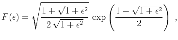 |
(18) |
and
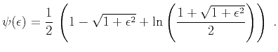 |
(19) |
The phase function  defined in equation A-7
corresponds to the analogous term in the exact-log DMO and AMO
(Liner, 1990; Zhou et al., 1996; Biondi and Vlad, 2002).
defined in equation A-7
corresponds to the analogous term in the exact-log DMO and AMO
(Liner, 1990; Zhou et al., 1996; Biondi and Vlad, 2002).
|
|
|
|
| OC-seislet: seislet transform construction with differential offset continuation | |
|
Next: Bibliography
Up: Liu and Fomel: OC-seislet
Previous: Conclusions
2013-03-02