|
|
|
|
Adaptive multiple subtraction using regularized nonstationary regression |
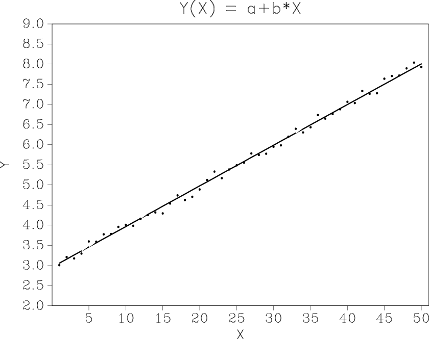
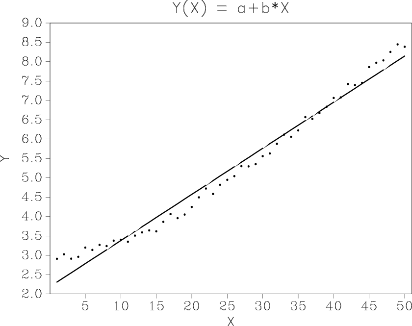
Figure 1a shows a classic example of linear regression applied as a line fitting problem. When the same technique is applied to data with a non-stationary behavior (Figure 1b), stationary regression fails to produce an accurate fit and creates regions of consistent overprediction and underprediction.
|
|---|
|
pred,pred2
Figure 1. Line fitting with stationary regression works well for stationary data (a) but poorly for non-stationary data (b). |
|
|
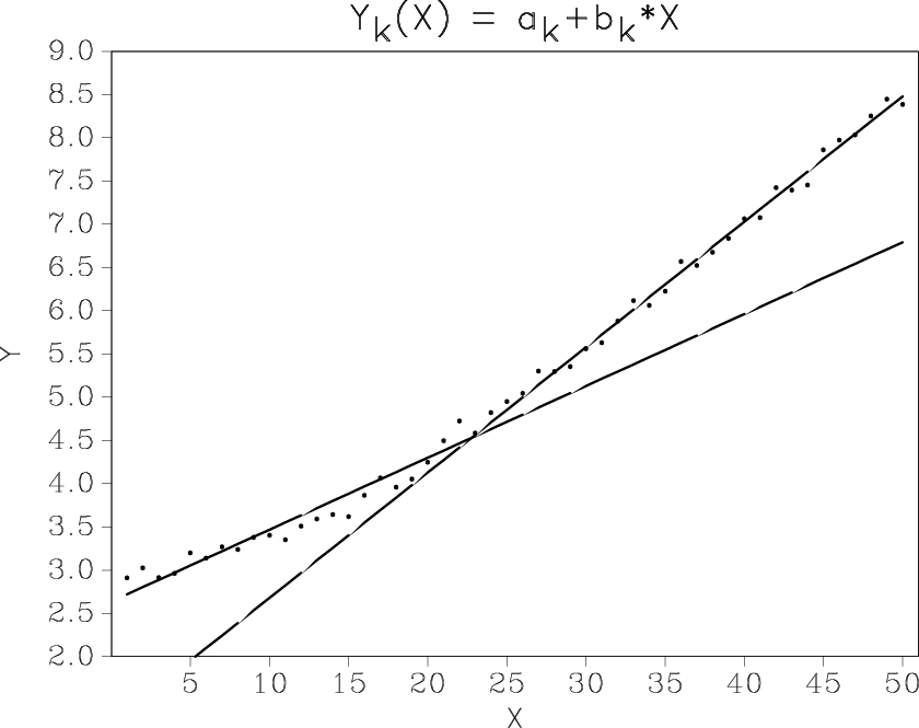
One remedy is to extend the model by including nonlinear terms (Figure 2a), another is to break the data into local windows (Figure 2b). Both solutions work to a certain extent but are not completely satisfactory, because they decreases the estimation stability and introduce additional non-intuitive parameters.
|
|---|
|
pred3,pred4
Figure 2. Nonstationary line fitting using nonlinear terms (a) and local windows (b). |
|
|
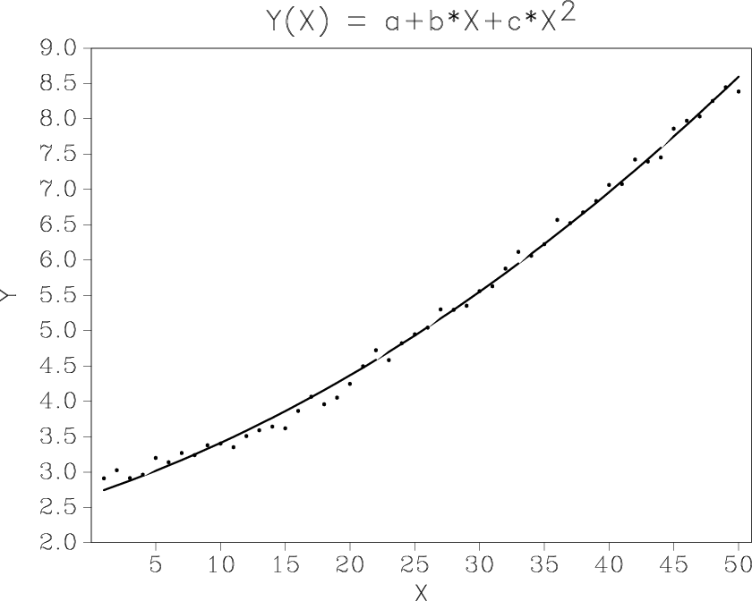
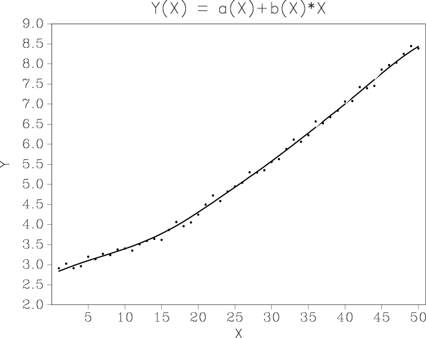
The regularized nonstationary solution, defined in the previous section, is shown in Figure 3. When using shaping regularization with smoothing as the shaping operator, the only additional parameter is the radius of the smoothing operator.
|
|---|
|
pred5
Figure 3. Nonstationary line fitting by regularized nonstationary regression. |
|
|
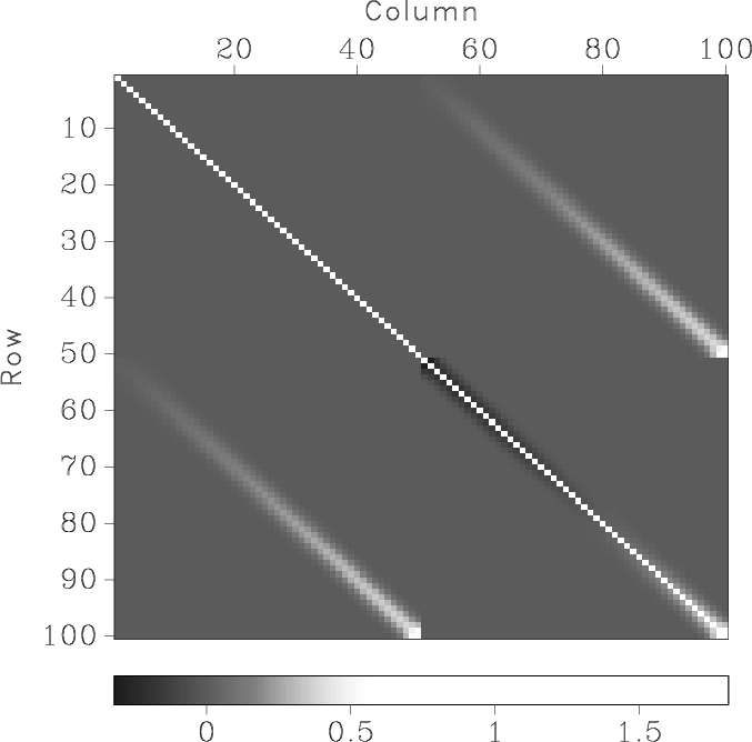
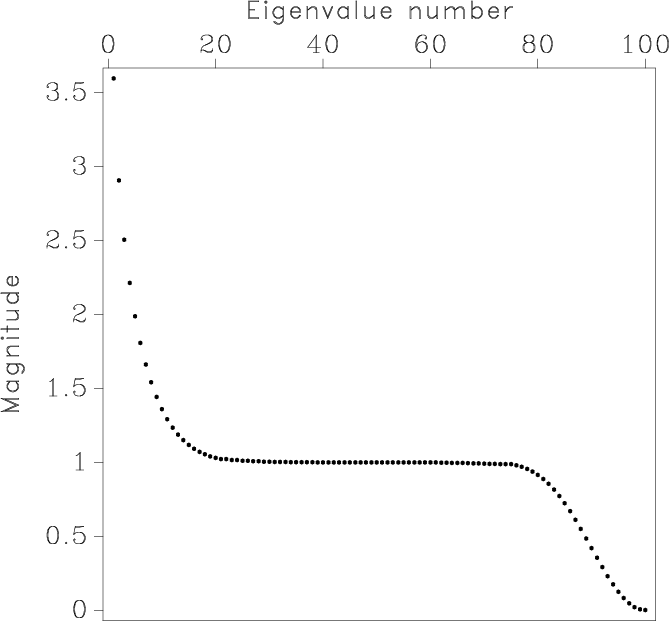
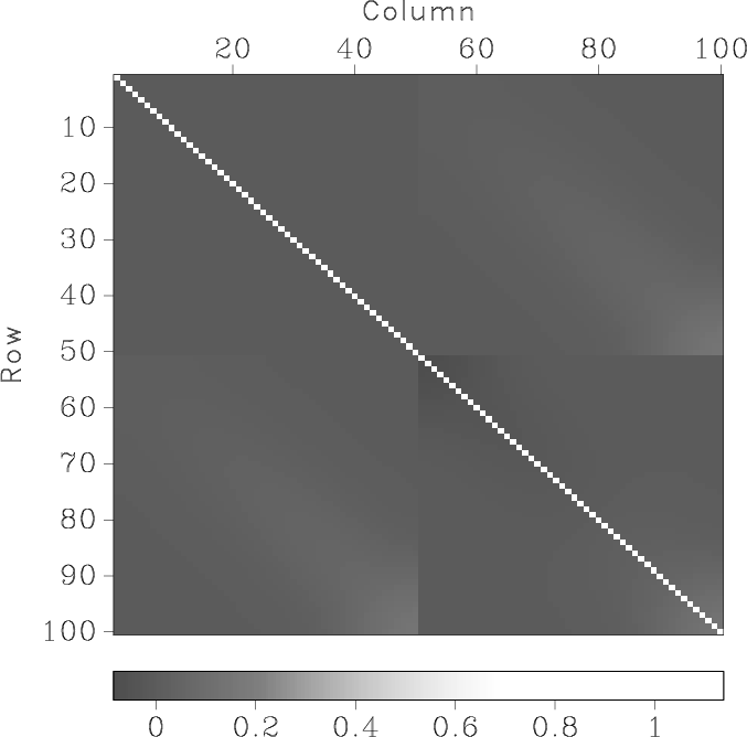
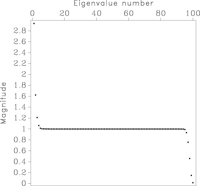
This toy example makes it easy to compare shaping regularization with
the more traditional Tikhonov's
regularization. Figures 4
and 5 show inverted matrix ![]() from
equation 5 and the distribution of its eigenvalues for two
different values of Tikhonov's regularization parameter
from
equation 5 and the distribution of its eigenvalues for two
different values of Tikhonov's regularization parameter ![]() ,
which correspond to mild and strong smoothing constraints. The
operator
,
which correspond to mild and strong smoothing constraints. The
operator ![]() in this case is the first-order
difference. Correspondingly, Figures 6
and 7 show matrix
in this case is the first-order
difference. Correspondingly, Figures 6
and 7 show matrix
![]() from
equation 7 and the distribution of its eigenvalues for
mild and moderate smoothing implemented with shaping. The operator
from
equation 7 and the distribution of its eigenvalues for
mild and moderate smoothing implemented with shaping. The operator
![]() is Gaussian smoothing controlled by the
smoothing radius.
is Gaussian smoothing controlled by the
smoothing radius.
When a matrix operator is inverted by an iterative method such as conjugate gradients, two characteristics control the number of iterations and therefore the cost of inversion (Golub and Van Loan, 1996; van der Vorst, 2003):
As the smoothing radius increases, matrix
![]() approaches the identity matrix, and the result of non-stationary
regression regularized by shaping approaches the result of stationary
regression. This intuitively pleasing behavior is difficult to emulate
with Tikhonov's regularization.
approaches the identity matrix, and the result of non-stationary
regression regularized by shaping approaches the result of stationary
regression. This intuitively pleasing behavior is difficult to emulate
with Tikhonov's regularization.
|
|---|
|
tmat0,teig0
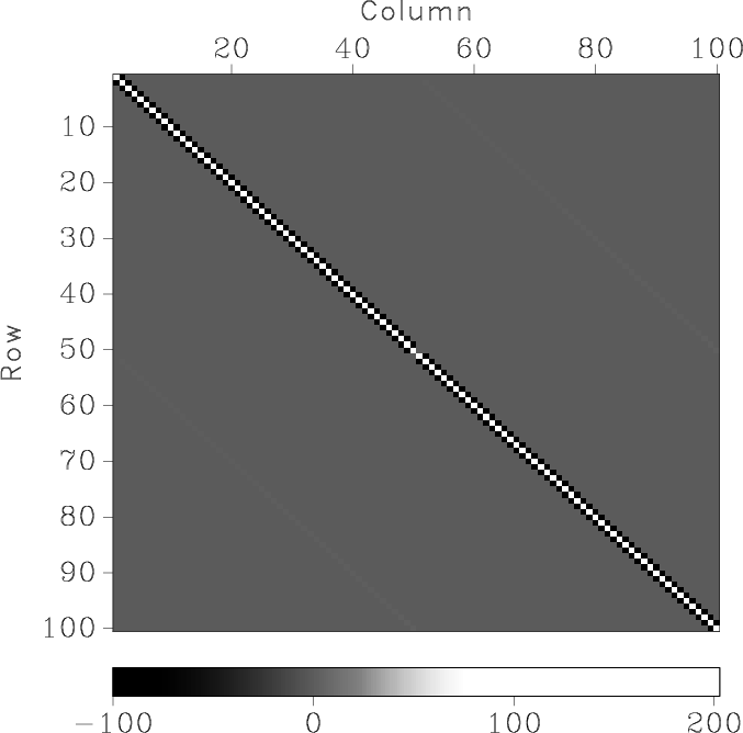
Figure 4. Matrix inverted in Tikhonov's regularization applied to nonstationary line fitting (a) and the distribution of its eigenvalues (b). The regularization parameter |
|
|

|
|---|
|
tmat2,teig2
Figure 5. Matrix inverted in Tikhonov's regularization applied to nonstationary line fitting (a) and the distribution of its eigenvalues (b). The regularization parameter |
|
|
|
|---|
|
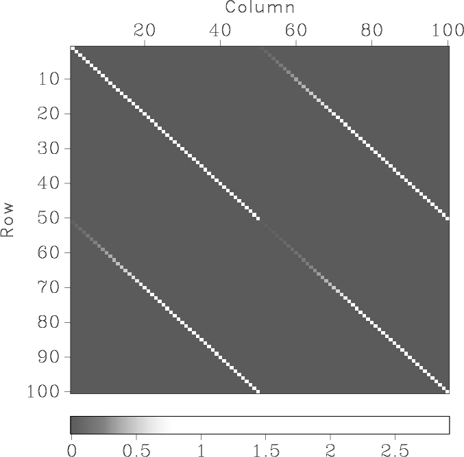
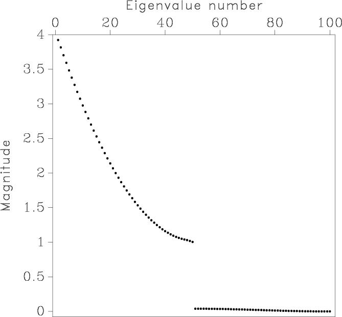
smat0,seig0
Figure 6. Matrix inverted in shaping regularization applied to nonstationary line fitting (a) and the distribution of its eigenvalues (b). The smoothing radius is 3 samples (mild smoothing). The condition number is |
|
|
|
|---|
|
smat1,seig1
Figure 7. Matrix inverted in shaping regularization applied to nonstationary line fitting (a) and the distribution of its eigenvalues (b). The smoothing radius is 15 samples (moderate smoothing). The condition number is |
|
|
|
|
|
|
Adaptive multiple subtraction using regularized nonstationary regression |