|
|
|
|
Seismic wave extrapolation using lowrank symbol approximation |
In this appendix, we outline the lowrank matrix approximation algorithm in more details.
Let ![]() be the number of samples both in space and wavenumber. Let
us denote the samples in the spatial domain by
be the number of samples both in space and wavenumber. Let
us denote the samples in the spatial domain by
![]() and the ones in the Fourier domain by
and the ones in the Fourier domain by
![]() . The elements of the interaction matrix
. The elements of the interaction matrix
![]() from equation (11) are then defined as
from equation (11) are then defined as
The first question is: which columns of
![]() shall one pick
for the matrix
shall one pick
for the matrix
![]() ? It has been shown by Goreinov et al. (1997)
and Gu and Eisenstat (1996) that the
? It has been shown by Goreinov et al. (1997)
and Gu and Eisenstat (1996) that the ![]() -dimensional volume spanned by
these columns should be the maximum or close to the maximum among all
possible choices of
-dimensional volume spanned by
these columns should be the maximum or close to the maximum among all
possible choices of ![]() columns from
columns from
![]() . More precisely, suppose
. More precisely, suppose
![]() is a column partitioning of
is a column partitioning of
![]() . Then one aims to find
. Then one aims to find
![]() such that
such that
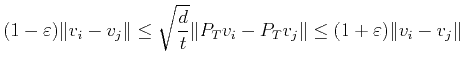
In order to overcome the problem associated with long vectors, the first idea is to project to a lower dimensional space and search for the set of vectors with maximum volume among the projected vectors. However, one needs to ensure that the volume is roughly preserved after the projection so that the set of vectors with the maximum projected volume also has a near-maximum volume in the original space. One of the most celebrated theorems in high dimensional geometry and probability is the following Johnson-Lindenstrauss lemma (Johnson and Lindenstrauss, 1984).
for
This theorem essentially says that projecting to a subspace of
dimension ![]() preserves the pairwise distance between
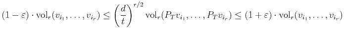
preserves the pairwise distance between ![]() arbitrary vectors. There is an immediate generalization of this
theorem due to Magen (2002), formulated
slightly differently for our purpose.
arbitrary vectors. There is an immediate generalization of this
theorem due to Magen (2002), formulated
slightly differently for our purpose.
for any
The main step of the proof is to bound the singular values of a random
matrix between
![]() and
and
![]() (after a uniform scaling) and this ensures that the
(after a uniform scaling) and this ensures that the ![]() -dimensional
volume is preserved within a factor of
-dimensional
volume is preserved within a factor of
![]() and
and
![]() . In order to obtain this bound on the singular
values, we need
. In order to obtain this bound on the singular
values, we need ![]() to be
to be
![]() . However, bounding the
singular values is only one way to bound the volume, hence it is
possible to improve the dependence of
. However, bounding the
singular values is only one way to bound the volume, hence it is
possible to improve the dependence of ![]() on
on ![]() . In fact, in
practice, we observe that
. In fact, in
practice, we observe that ![]() only needs to scale like
only needs to scale like
![]() .
.
Given a generic subspace ![]() of dimension
of dimension ![]() , computing the
projections
, computing the
projections
![]() takes
takes ![]() steps. Recall
that our goal is to find an algorithm with linear complexity, hence
this is still too costly. In order to reduce the cost of the random
projection, the second idea of our approach is to randomly choose
steps. Recall
that our goal is to find an algorithm with linear complexity, hence
this is still too costly. In order to reduce the cost of the random
projection, the second idea of our approach is to randomly choose ![]() coordinates and then project (or restrict) each vector only to these
coordinates. This is a projection with much less randomness but one
that is much more efficient to apply. Computationally, this is
equivalent to restricting
coordinates and then project (or restrict) each vector only to these
coordinates. This is a projection with much less randomness but one
that is much more efficient to apply. Computationally, this is
equivalent to restricting
![]() to
to ![]() randomly selected
rows. We do not yet have a theorem regarding the volume for this
projection. However, it preserves the
randomly selected
rows. We do not yet have a theorem regarding the volume for this
projection. However, it preserves the ![]() -dimensional volume very well
for the matrix
-dimensional volume very well
for the matrix
![]() and this is in fact due to the oscillatory
nature of the columns of
and this is in fact due to the oscillatory
nature of the columns of
![]() . We denote the resulting vectors by
. We denote the resulting vectors by
![]() .
.
The next task is to find a set of columns
![]() so
that the volume
so
that the volume
![]() is
nearly maximum. As we mentioned earlier, exhaustive search is too
costly. To overcome this, the third idea is to use the following
pivoted QR algorithm (or pivoted Gram-Schmidt process) to find the
is
nearly maximum. As we mentioned earlier, exhaustive search is too
costly. To overcome this, the third idea is to use the following
pivoted QR algorithm (or pivoted Gram-Schmidt process) to find the ![]() columns.
columns.
![\begin{algorithmic}[1]
\FOR{$s=1,\ldots, r$}
\par
\STATE Find $j_s$ among $\{1...
...R
\par
\STATE $\{j_1,\ldots,j_r\}$ is the column set required
\end{algorithmic}](img128.png)
Once the column set is found, we set
![]() .
.
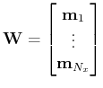
In order to identify
![]() , one needs to find a set of
, one needs to find a set of ![]() rows of
rows of
![]() that has an almost maximum volume. To do that, we repeat the same
steps now to
that has an almost maximum volume. To do that, we repeat the same
steps now to
![]() . More precisely, let
. More precisely, let
![\begin{algorithmic}
% latex2html id marker 425
[1]
\STATE Select uniform random...
...\vdots\\
\mathbf{m}_{i_r}
\end{bmatrix}\;.
\end{equation}\end{algorithmic}](img132.png)
Once both
![]() and
and
![]() are identified, the last task is to compute
the
are identified, the last task is to compute
the ![]() matrix
matrix
![]() for
for
![]() . Minimizing
. Minimizing
Let us now discuss the overall cost of this algorithm. Random sampling
of ![]() rows and
rows and ![]() columns of the matrix
columns of the matrix
![]() clearly takes
clearly takes ![]() steps. Pivoted QR factorization on the projected columns
steps. Pivoted QR factorization on the projected columns
![]() takes
takes
![]() steps and the cost for
for the pivoted QR factorization on the projected rows. Finally,
performing pseudo-inverses takes
steps and the cost for
for the pivoted QR factorization on the projected rows. Finally,
performing pseudo-inverses takes ![]() steps. Therefore, the
overall cost of the algorithm is
steps. Therefore, the
overall cost of the algorithm is
![]() .
As we mentioned earlier, in practice
.
As we mentioned earlier, in practice
![]() . Hence, the
overall cost is linear in
. Hence, the
overall cost is linear in ![]() .
.
|
|
|
|
Seismic wave extrapolation using lowrank symbol approximation |