 |
 |
 |
 | Generalized nonhyperbolic moveout approximation |  |
![[pdf]](icons/pdf.png) |
Next: Connection with other approximations
Up: Fomel & Stovas: Generalized
Previous: INTRODUCTION
Let  represent the reflection traveltime as a function of the
source-receiver offset
represent the reflection traveltime as a function of the
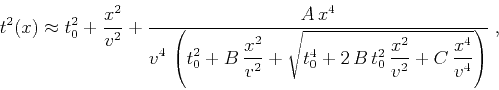
source-receiver offset  . We propose the following general form of
the moveout approximation:
. We propose the following general form of
the moveout approximation:
 |
(1) |
The five parameters  ,
,  ,
,  ,
,  , and
, and  describe the moveout behavior. By simple algebraic manipulations, one
can also rewrite equation 1 as
describe the moveout behavior. By simple algebraic manipulations, one
can also rewrite equation 1 as
 |
(2) |
where the new set of parameters  ,
,  ,
,  ,
,  , and is
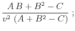
related to the previous set by the equalities
, and is
related to the previous set by the equalities
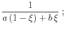
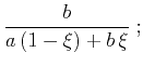
The inverse transform is given by
The existence of the nonhyperbolic part in the traveltime
approximation 1 and 2 is controlled by parameter
. When is zero (which implies that  or
or  ),
approximation 1 is hyperbolic. When both and are
very large, approximation 2 also reduces to the hyperbolic
form.
),
approximation 1 is hyperbolic. When both and are
very large, approximation 2 also reduces to the hyperbolic
form.
Subsections
|
|
|
|
| Generalized nonhyperbolic moveout approximation | |
|
Next: Connection with other approximations
Up: Fomel & Stovas: Generalized
Previous: INTRODUCTION
2013-03-02

![$\displaystyle \frac{\xi\,\left(c - b^2\right)}
{\left[a\,(1-\xi) + b\,\xi\right]^2}\;;$](img31.png)
![$\displaystyle \frac{c}{\left[a\,(1-\xi) + b\,\xi\right]^2}\;.$](img35.png)