 |
 |
 |
 | Kirchhoff migration using eikonal-based computation of traveltime source-derivatives |  |
![[pdf]](icons/pdf.png) |
Next: Numerical Examples
Up: Theory and Implementation
Previous: Traveltime Source-derivative
Equation 6 is a linear first-order PDE suitable for upwind numerical methods
(Franklin and Harris, 2001). Since it does not change the non-linear nature of the eikonal equation,
the resulting traveltime source-derivative can be related to any branch of multi-arrivals,
if one supplies the corresponding traveltime in  . The source-derivatives can be
computed either along with traveltimes or separately. In Appendix A, we describe a first-arrival
implementation based on a modification of FMM (Sethian, 1996).
. The source-derivatives can be
computed either along with traveltimes or separately. In Appendix A, we describe a first-arrival
implementation based on a modification of FMM (Sethian, 1996).
The first-order traveltime source-derivative enables a cubic Hermite interpolation
(Press et al., 2007). Geometrically, such an interpolation is valid only when the selected
wave-front in the interpolation interval is smooth and continuous. For a 2D model and a
source interpolation along the inline direction only, the Hermite interpolation reads:
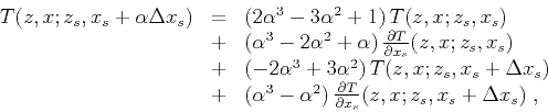 |
(10) |
where
![$\alpha \in [0,1]$](img54.png) controls the source position to be interpolated between known
values at
controls the source position to be interpolated between known
values at  and
and
 . For comparison, the linear interpolation
can be represented by:
. For comparison, the linear interpolation
can be represented by:
 |
(11) |
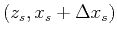
The linear interpolation fixes the subsurface image point  . A possible
improvement is to instead fix the vector that links the source with the image, such
that on the right-hand side the traveltimes are taken at shifted image locations:
. A possible
improvement is to instead fix the vector that links the source with the image, such
that on the right-hand side the traveltimes are taken at shifted image locations:
 |
(12) |
We will refer to scheme 12 as shift interpolation. According to our definition
of the relative coordinate  in equation 2, shift interpolation
amounts to a linear interpolation in
in equation 2, shift interpolation
amounts to a linear interpolation in
 . It is easy to verify
that, for a constant-velocity medium, both Hermite and shift interpolations are accurate,
while the linear interpolation is not. However, the accuracy of shift interpolation deteriorates
with increasing velocity variations, as it assumes that the wave-front remains invariant in
the relative coordinate. Equations 10-12 can be generalized to 3D by
cascading the inline and crossline interpolations (for example equation 11 in 3D
case becomes bilinear interpolation). The interpolated source does not need to lie collinear
with source samples.
. It is easy to verify
that, for a constant-velocity medium, both Hermite and shift interpolations are accurate,
while the linear interpolation is not. However, the accuracy of shift interpolation deteriorates
with increasing velocity variations, as it assumes that the wave-front remains invariant in
the relative coordinate. Equations 10-12 can be generalized to 3D by
cascading the inline and crossline interpolations (for example equation 11 in 3D
case becomes bilinear interpolation). The interpolated source does not need to lie collinear
with source samples.
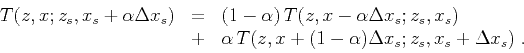
The derivatives themselves can also be directly used for Kirchhoff anti-aliasing
(Lumley et al., 1994; Abma et al., 1999; Fomel, 2002). Equations 10, 11
and 12 give rise to their corresponding source-derivative interpolations
after applying the following chain-rule to both sides:
 |
(13) |
The anti-aliasing application is summarized in Appendix B.
|
|
|
|
| Kirchhoff migration using eikonal-based computation of traveltime source-derivatives | |
|
Next: Numerical Examples
Up: Theory and Implementation
Previous: Traveltime Source-derivative
2013-06-24