 |
 |
 |
 | Non-hyperbolic common reflection surface |  |
![[pdf]](icons/pdf.png) |
Next: Accuracy comparisons
Up: Hyperbolic and nonhyperbolic CRS
Previous: Hyperbolic and nonhyperbolic CRS
In the case of 3-D multi-azimuth acquisition, both  and
and  become
two-dimensional vectors. A natural way to extend
approximation (8) is to replace it with
become
two-dimensional vectors. A natural way to extend
approximation (8) is to replace it with
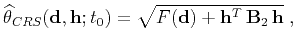 |
(14) |
where
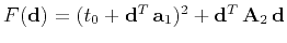 ,
,
 is a
two-dimensional vector, and
is a
two-dimensional vector, and
 and
and
 are
two-by-two symmetric matrices (Tygel and Santos, 2007). A similar approach
works for extending approximation (12) to
are
two-by-two symmetric matrices (Tygel and Santos, 2007). A similar approach
works for extending approximation (12) to
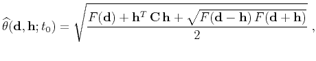 |
(15) |
where
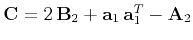 .
In the 3-D case, we have not found a simple connection between
approximation (15) and the analytical reflection
traveltime for a 3-D hyperbolic reflector.
.
In the 3-D case, we have not found a simple connection between
approximation (15) and the analytical reflection
traveltime for a 3-D hyperbolic reflector.
2013-03-02