|
|
|
|
Seismic data interpolation beyond aliasing using regularized nonstationary autoregression |
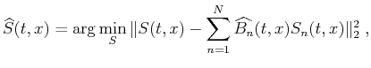
In the second step, a similar problem is solved, except that the filter is known, and the missing traces are unknown. In the decimated-trace interpolation problem, we squeeze (by throwing away alternate zeroed rows and columns) the filter in equation 3 to its original size and then formulate the least-squares problem,
We carry out the minimization in
equations 4, 13, and 14 by the
conjugate gradient method (Hestenes and Stiefel, 1952). The constraint
condition (equation 15) is used as the initial model and
constrains the output by using the known traces for each iteration in
the conjugate-gradient scheme. The computational cost is proportional to
![]() , where
, where ![]() is the number of iterations,
is the number of iterations, ![]() is the filter size, and
is the filter size, and
![]() is the data size. In our tests,
is the data size. In our tests, ![]() and
and ![]() were
approximately equal to 100. Increasing the smoothing radius in shaping
regularization decreases
were
approximately equal to 100. Increasing the smoothing radius in shaping
regularization decreases ![]() in the filter estimation step.
in the filter estimation step.
|
|
|
|
Seismic data interpolation beyond aliasing using regularized nonstationary autoregression |