Theory of 3-D angle gathers in wave-equation seismic imaging

Common-azimuth approximation

Common-azimuth migration (Biondi and Palacharla, 1996) is a downward continuation imaging method tailored for narrow-azimuth streamer surveys that can be transformed to a single common azimuth with the help of azimuth moveout (Biondi et al., 1998) Employing the common-azimuth approximation, one assumes the reflection plane stays confined in the acquisition azimuth. Although this assumption is strictly valid only in the case of constant velocity (Vaillant and Biondi, 2000), the modest azimuth variation in realistic situations justifies the use of the method (Biondi, 2003).

To restrict equations of the previous section to the common-azimuth approximation, it is sufficient to set the cross-line offset $h_y$ to zero assuming the $x$ coordinate is oriented along the acquisition azimuth. In particular, from equations (8-9), we obtain

$$h_x\,\sin{\alpha} = \frac{v\,t}{2}\,\sin{\theta}$$ (19)

$$t_{h_x} = \frac{4\,h_x}{v^2\,t}\,\sin^2{\alpha} = \frac{2}{v}\,\sin{\theta}\,\sin{\alpha}\;,$$ (20)

$$t_{h_y} = -\frac{4\,h_x}{v^2\,t}\,\cos{\alpha}\,\cos{\beta} = - \frac{2}{v}\,\sin{\theta}\,\cot{\alpha}\,\cos{\beta}\;.$$ (21)

With the help of equations (6), (7), and (10), equation (21) transforms to the form

$$t_{h_y} = t_{m_y}\,\frac{\tan{\theta}}{\tan{\alpha}}$$

$$= t_{m_y}\,\frac{ \sqrt{1-\frac{v^2}{4}\,\left(t_{m_x}+t_{h_x}\rig... ...t_{h_x}\right)^2} + \sqrt{1-\frac{v^2}{4}\,\left(t_{m_x}-t_{h_x}\right)^2}}\;,$$ (22)

suggested by Biondi and Palacharla (1996). Combining equations (6), (7), (10), and (20) and transforming to the frequency-wavenumber domain, we obtain the common-azimuth dispersion relationship

$$\left(k_{h_x}^2 + k_{m_y}^2 + k_z^2\right)\, \left(k_{m_x}^2 + k_... ...}^2 + k_z^2\right) = \frac{4\,\omega^2}{v^2}\,\left(k_{m_y}^2 + k_z^2\right)\;,$$ (23)

which shows that, under the common-azimuth approximation and in a laterally homogeneous medium, 3-D seismic migration amounts to a cascade of a 2-D prestack migrations in the in-line direction and a 2-D zero-offset migration in the cross-line direction (Canning and Gardner, 1996).

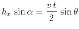
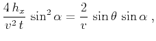
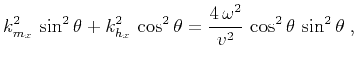
Under the common-azimuth approximation, the angle-dependent relationship (13) takes the form

$$k_{m_x}^2\,\sin^2{\theta} + k_{h_x}^2\,\cos^2{\theta} = \frac{4\,\omega^2}{v^2}\,\cos^2{\theta}\,\sin^2{\theta}\;,$$ (24)

which is identical to the 2-D equation (14). This proves that under this approximation, one can perform the structural correction independently for each cross-line wavenumber.

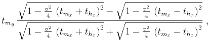
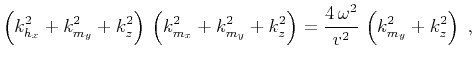
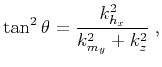
The post-imaging equation (16) transforms to the equation

$$\tan^2{\theta} = \frac{k_{h_x}^2}{k_{m_y}^2 + k_z^2}\;,$$ (25)

obtained previously by Biondi et al. (2003). In the absence of cross-line structural dips ($k_{m_y}=0$ ), it is equivalent to the 2-D equation (18).

Theory of 3-D angle gathers in wave-equation seismic imaging