|
|
|
|
Seismic data interpolation without iteration using |
To evaluate the performance of the ![]() -
-![]() -
-![]() SPF interpolation
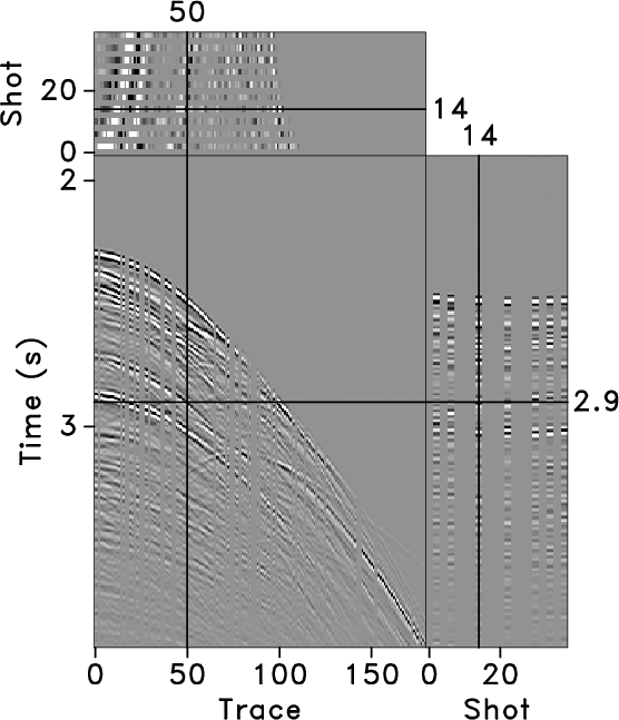
method in 3D field conditions, we chose a set of marine shot gathers
from a deep-water Gulf of Mexico survey
(Liu and Fomel, 2011; Fomel, 2002). Figure 8a shows the complicated
diffraction events caused by a salt body. We selected
SPF interpolation
method in 3D field conditions, we chose a set of marine shot gathers
from a deep-water Gulf of Mexico survey
(Liu and Fomel, 2011; Fomel, 2002). Figure 8a shows the complicated
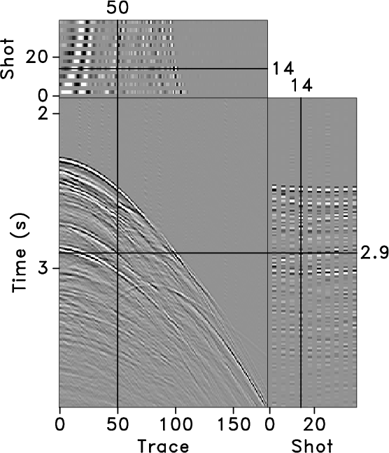
diffraction events caused by a salt body. We selected ![]() traces
of the input data by subsampling in the shot direction and removing
traces
of the input data by subsampling in the shot direction and removing
![]() random traces (Figure 8b). For comparison, we
used 3D Fourier POCS method and the conventional SPF to
reconstruct the missing traces (Figure 9a
and 9b, respectively). The Fourier POCS method
also failed to interpolate the decimated traces and created some
artificial events at the locations of the randomly-missing traces. The
interpolated result could be partially improved by slicing data into
patching windows. The conventional 3D
random traces (Figure 8b). For comparison, we
used 3D Fourier POCS method and the conventional SPF to
reconstruct the missing traces (Figure 9a
and 9b, respectively). The Fourier POCS method
also failed to interpolate the decimated traces and created some
artificial events at the locations of the randomly-missing traces. The
interpolated result could be partially improved by slicing data into
patching windows. The conventional 3D ![]() -
-![]() -
-![]() SPF also failed to
recover the decimated data. Figure 9c shows
that the proposed
SPF also failed to
recover the decimated data. Figure 9c shows
that the proposed ![]() -
-![]() -
-![]() SPF method produced better result, in
which the missing gaps were recovered reasonable well, except for
weaker amplitude in the common-offset sections.
Figure 10 provides the
SPF method produced better result, in
which the missing gaps were recovered reasonable well, except for
weaker amplitude in the common-offset sections.
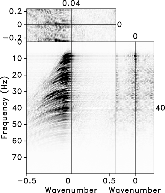
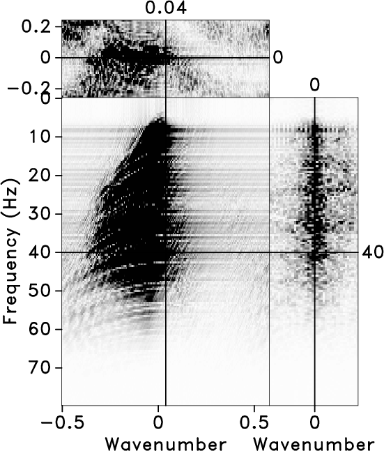
Figure 10 provides the ![]() -
-![]() spectra corresponding to the original data and interpolated results
with the Fourier POCS, the conventional 3D
spectra corresponding to the original data and interpolated results
with the Fourier POCS, the conventional 3D ![]() -
-![]() -
-![]() SPF, and the
proposed 3D
SPF, and the
proposed 3D ![]() -
-![]() -
-![]() SPF,
respectively. Figure 11 show the
interpolation errors using these methods. The simultaneous occurrence
of regular and irregular data missing is a challenge in the
interpolation process. The proposed 3D
SPF,
respectively. Figure 11 show the
interpolation errors using these methods. The simultaneous occurrence
of regular and irregular data missing is a challenge in the
interpolation process. The proposed 3D ![]() -
-![]() -
-![]() SPF method shows
more reasonable results than the Fourier POCS and the conventional
streaming PEF. Meanwhile, the proposed algorithm is more efficient,
and the CPU times for the 3D POCS with 500 iterations was 380.42 s
whereas those of the 3D
SPF method shows
more reasonable results than the Fourier POCS and the conventional
streaming PEF. Meanwhile, the proposed algorithm is more efficient,
and the CPU times for the 3D POCS with 500 iterations was 380.42 s
whereas those of the 3D ![]() -
-![]() -
-![]() SPF was 12.27 s.
SPF was 12.27 s.

|
|---|
|
s3,m3
Figure 8. (a) A 3D field dataset and (b) data after subsampling in the shot direction and |
|
|


|
|---|
|
pocsqd,adds,a3
Figure 9. Interpolated results using different methods. (a) The 3D Fourier POCS, (b) the conventional 3D |
|
|


|
|---|
|
seanfk,pocsfk,addsfk,addfk
Figure 10. The |
|
|


|
|---|
|
errpocsqd,difs,ds3
Figure 11. Interpolation errors using different methods. (a) The 3D Fourier POCS, (b) the conventional 3D |
|
|
|
|
|
|
Seismic data interpolation without iteration using |