|
|
|
|
Adaptive prediction filtering in |

|
|---|
|
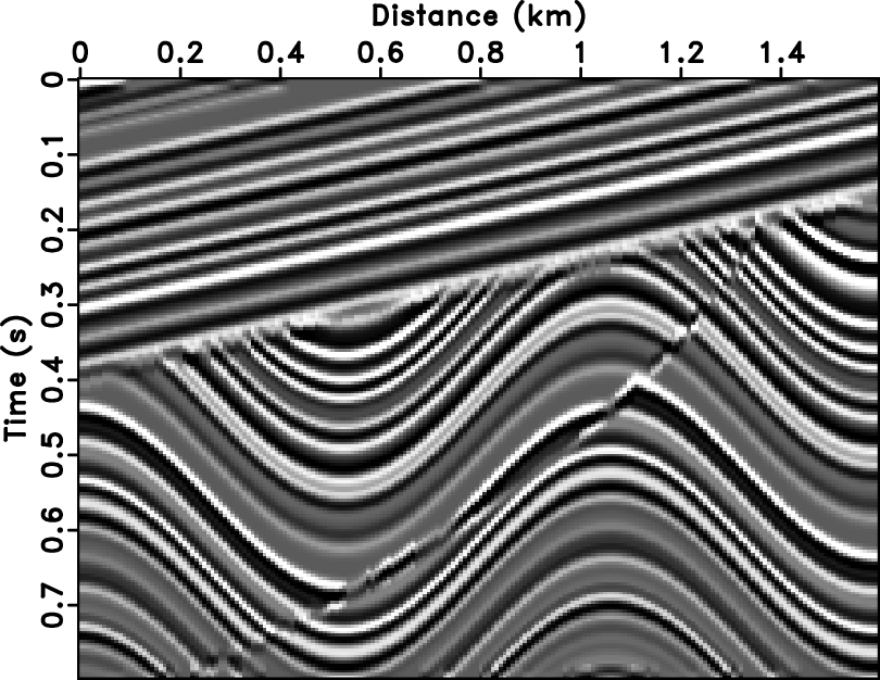
sigmoid,noise
Figure 7. 2D poststack model (a) and noisy data (b). |
|
|


|
|---|
|
sfxrna,sfxnoiz,apfs,apfn
Figure 8. Comparison of nonstationary methods. The denoised result by |
|
|
|
|
|
|
Adaptive prediction filtering in |