Streaming orthogonal prediction filter in $t$ -$x$ domain for random noise attenuation

theory

In the $t$ -$x$ domain, seismic data always display native nonstationarity. However, one can assume that the new prediction filter $\mathbf{a}$ stays close to the previous filter on time axis $\bar{\mathbf{a}}_t$ and the previous filter on space axis $\bar{\mathbf{a}}_x$ . The autoregression equation of the $t$ -$x$ streaming PF can be written in a shortened block-matrix notation (Fomel and Claerbout, 2016) as

$$\left[ \begin{array}{c} \mathbf{d}^T\\ \lambda_t \mathbf{I}\\ \la... ...\lambda_t \mathbf{\bar{a}}_t\\ \lambda_x \mathbf{\bar{a}}_x \end{array}\right],$$ (1)

where $\mathbf{I}$ is the identity matrix and $d(t,x)$ is the given data sample at the point $(t,x)$ . $\lambda_t$ and $\lambda_x$ are the scale parameters controlling the filter variability on the two axes.

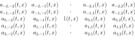
Consider a 2D noncausal prediction filter with 20 prediction coefficients $a_{i,j}$ :

$$\begin{array}{ccccc} a_{-2,-2}(t,x) & a_{-2,-1}(t,x) & \cdot ... ...a_{2,-1}(t,x) & \cdot & a_{2,1}(t,x) & a_{2,2}(t,x) \end{array}$$ (2)

where ``$\cdot$ '' denotes zero, and the data vector $\mathbf{d}$ and the filter vector $\mathbf{a}$ in equation 1 are shown as follows:

$$\mathbf{d}=\left[ \begin{array}{c} d_{-M,-N}(t,x)\\ d_{-M+1,-N}(t... ...\ a_{-M+1,-N}(t,x)\\ \ldots\\ a_{M-1,N}(t,x)\\ a_{M,N}(t,x) \end{array}\right],$$ (3)

where $d_{i,j}(t,x)$ represents the translation of $d(t,x)$ in both time and space directions with time shift $i$ and space shift $j$ . $2M+1$ and $2N$ are the temporal and spatial lengths of the prediction filter, e.g., $M$ =2 and $N$ =2 in equation 2.

The least-squares solution of equation 1 is

$$\mathbf{a}=(\mathbf{d}\mathbf{d}^T+\lambda^2\mathbf{I})^{-1}(-d(t,x) \mathbf{d}+\lambda^2\mathbf{\bar{a}}),$$ (4)

where

$$\lambda^2=\lambda_t^2+\lambda_x^2, \quad\mathbf{\bar{a}}=\frac{\l... ...t^2\mathbf{\bar{a}}_t+ \lambda_x^2\mathbf{\bar{a}}_x}{\lambda_t^2+\lambda_x^2}.$$ (5)

Fomel and Claerbout (2016) propose the Sherman-Morrison formula to directly transform the inverse matrix in equation 4 without iterations. The Sherman-Morrison formula is an analytic method for solving the inverse of a special matrix (Hager, 1989). If both matrices $\mathbf{A}$ and $\mathbf{I}-\mathbf{V}\mathbf{A}^{-1}\mathbf{U}$ are invertible, then $\mathbf{A}-\mathbf{U}\mathbf{V}$ is invertible and

$$(\mathbf{A}-\mathbf{U}\mathbf{V})^{-1}=\mathbf{A}^{-1}+ \mathbf{A... ...\mathbf{I}- \mathbf{V}\mathbf{A}^{-1}\mathbf{U})^{-1}\mathbf{V}\mathbf{A}^{-1}.$$ (6)

In the special case where matrix $\mathbf{U}$ is a column vector $\mathbf{u}$ and matrix $\mathbf{V}$ is a row vector $\mathbf{v}$ , equation 6 can be rewritten as

$$(\mathbf{A}-\mathbf{u}\mathbf{v})^{-1}=\mathbf{A}^{-1}+ \mathbf{A... ...athbf{u}(1- \mathbf{v}\mathbf{A}^{-1}\mathbf{u})^{-1}\mathbf{v}\mathbf{A}^{-1}.$$ (7)

The direct derivation of the Sherman-Morrison formula (equation 7) is described in Appendix A.

Applying the Sherman-Morrison formula to equation 4, the $t$ -$x$ streaming PF coefficients and prediction error can be calculated as

$$\mathbf{a}=\mathbf{\bar{a}}-\left(\frac{d(t,x)+\mathbf{d}^T\mathbf{\bar{a}}} {\lambda^2+\mathbf{d}^T\mathbf{d}}\right)\mathbf{d},$$ (8)

and

$$r(t,x)=\frac{\lambda^2(d(t,x)+\mathbf{d}^T\mathbf{\bar{a}})} {\lambda^2+\mathbf{d}^T\mathbf{d}}.$$ (9)

For seismic random noise attenuation, we assume the residual of prediction filtering $r(t,x)$ is the random noise at the point $(t,x)$ . For calculating 2D $t$ -$x$ streaming PFs, we need to store one previous time-neighboring PF, $\mathbf{\bar{a}}_t$ , and one previous space-neighboring PF, $\mathbf{\bar{a}}_x$ , both $\mathbf{\bar{a}}_t$ and $\mathbf{\bar{a}}_x$ will be used when the stream arrives at its adjacency.

One can compare a streaming PF with a stationary PF. The autoregression equation for a traditional PF takes the following form:

$$d(t,x)+\sum_{j=-N,j\neq0}^{j=N}\sum_{i=-M}^{i=M}a_{i,j}d_{i,j}(t,x) \approx 0.$$ (10)

The least-squares solution of equation 10 at each point $(t,x)$ is

$$\mathbf{a}=-d(t,x)(\mathbf{d}\mathbf{d}^T)^{-1}\mathbf{d}.$$ (11)

The matrix in equation 11 is similar to that in equation 4. The comparison of equation 4 and equation 11 indicates that the results of the streaming PFs become gradually more accurate as the scale parameter $\lambda$ decreases. However, according to equation 9, a small $\lambda$ may cause the residual $r(t,x)$ to also be small, which means that there is too much noise in the signal section. To solve this problem, we use a two-step strategy. First, we choose a relatively large $\lambda$ to get a large residual $r(t,x)$ . The first step amounts to an ``over-filtering'', which generates an approximately ``clean'' signal. Next, the signal leakage in the noise section can be extracted by applying signal-and-noise orthogonalization.

We derive the definition of the streaming orthogonalization weight (SOW) from the global orthogonalization weight (GOW) (Chen and Fomel, 2015). Assume that the leaking signal $\mathbf{s}_1$ has a linear correlation with the estimated signal section $\mathbf{s}_0$ in the first step,

$$\mathbf{s}_1=\omega\mathbf{s}_0,$$ (12)

where $\omega$ is the GOW. The ideal signal $\mathbf{s}$ and noise $\mathbf{n}$ can then be estimated by

$$\mathbf{s}=\mathbf{s}_0+\omega\mathbf{s}_0,$$ (13)

$$\mathbf{n}=\mathbf{n}_0-\omega\mathbf{s}_0.$$ (14)

Under the assumption that the noise $\mathbf{n}$ is orthogonal to the signal $\mathbf{s}$ ,

$$\mathbf{n}^T\mathbf{s}=0.$$ (15)

Substituting equation 13 and 14 into equation 15, one can get the GOW as

$$\omega=\frac{\mathbf{n}_0^T\mathbf{s}_0}{\mathbf{s}_0^T\mathbf{s}_0}.$$ (16)

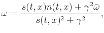
To get the orthogonalization weight for each data value, one possible definition of the SOW is:

$$\omega(t,x)=\frac{s(t,x)n(t,x)}{s(t,x)^2}=\frac{n(t,x)}{s(t,x)},$$ (17)

where $\omega(t,x)$ is the SOW for the data point $d(t,x)$ . $s(t,x)$ and $n(t,x)$ represent the signal and noise values at the point $(t,x)$ , respectively. In the SOPF, $s(t,x)$ and $n(t,x)$ correspond to the predictable part $\mathbf{d}^T\mathbf{a}$ and the prediction residual $r(t,x)$ produced in the first step. Direct point-by-point division of the values may produce unstable values. One common method to solve this problem is the iterative least-squares method (Chen and Fomel, 2015). Here, we propose a streaming method to calculate the SOW.

Suppose that the SOW gets updated with each new data point $d(t,x)$ . The new SOW, $\omega$ , should stay close to the previous time-neighboring SOW $\bar{\omega}_t$ and the previous space-neighboring SOW $\bar{\omega}_x$ . Equation 17 can be rewritten as

$$\left[ \begin{array}{c} s(t,x)\\ \gamma_t\\ \gamma_x \end{array}\... ...c} n(t,x)\\ \gamma_t\bar{\omega}_t\\ \gamma_x\bar{\omega}_x \end{array}\right],$$ (18)

where $\gamma_t$ and $\gamma_x$ are the scale parameters controlling the variability on the two axes.

The least-squares solution of equation 18 is

$$\omega=\frac{s(t,x)n(t,x)+\gamma^2\bar{\omega}}{s(t,x)^2+\gamma^2},$$ (19)

where

$$\gamma^2=\gamma_t^2+\gamma_x^2, \quad\bar{\omega}=\frac{\gamma_t^2\bar{\omega}_t+\gamma_x^2\bar{\omega}_x} {\gamma_t^2+\gamma_x^2}.$$ (20)

Applying equation 13, one can get the denoised data value $\hat{s}(t,x)$ after the SOPF

$$\hat{s}(t,x)=s(t,x)+\frac{s(t,x)r(t,x)+\gamma^2\bar{\omega}} {s(t,x)^2+\gamma^2}s(t,x),$$ (21)

where $s(t,x)$ and $r(t,x)$ are the predictable signals and the prediction residuals calculated in the first step.

We implement the two-step strategy within the streaming method and obtain the denoised data value as each new noisy data value arrives. Table 1 compares the computational cost between $f$ -$x$ deconvolution, $f$ -$x$ regularized nonstationary autoregression (RNA) (Liu et al., 2012), and the proposed method. In general, the cost of SOPF is minimal.

Method	Filter storage	Cost
$f$ -$x$ deconvolution	$O(N_a)$	$O(N_a N_f N_x N_{iter})$
$f$ -$x$ RNA	$O(N_a N_f N_x)$	$O(N_a N_f N_x N_{iter})$
$t$ -$x$ SOPF	$O(N_a N_t)$	$O(N_a N_t N_x)$

Table 1. Rough cost comparison between $f$ -$x$ deconvolution, $f$ -$x$ RNA, and $t$ -$x$ SOPF. $N_a$ is the filter size, $N_f$ is the frequency size of the data in frequency domain, $N_x$ is the spatial size of the data, $N_t$ is the temporal size of the data, and $N_{iter}$ is the number of iterations.

Streaming orthogonal prediction filter in $t$ -$x$ domain for random noise attenuation