|
 |
 |
 | Noniterative f-x-y streaming prediction filtering for random noise attenuation on seismic data |  |
![[pdf]](icons/pdf.png) |
Next: Data processing path in
Up: Theory
Previous: Theory
A 2D seismic section  containing linear events can be
described as a plane wave function in the
containing linear events can be
described as a plane wave function in the  -
- domain. In the
 -
domain, the linear events in seismic section
-
domain, the linear events in seismic section
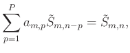
 are decomposed into a series of sinusoids. These sinusoids are
superimposed and become harmonics at each frequency, which shows the
prediction relationship of seismic traces in a frequency slice:
are decomposed into a series of sinusoids. These sinusoids are
superimposed and become harmonics at each frequency, which shows the
prediction relationship of seismic traces in a frequency slice:
 |
(1) |
where
![$ m \in [1,M]$](img11.png) and
and
![$ n \in [1,N]$](img12.png) are the indices of the seismic
sample along the
axis and
axis, respectively.
are the indices of the seismic
sample along the
axis and
axis, respectively.
![$ p \in [1,P]$](img13.png) is
the index of filter coefficients along the
direction.
is
the index of filter coefficients along the
direction.
 denotes the data point in
and
denotes the data point in
and
 indicates the filter coefficient in the
-
domain. When
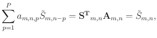
curve events or amplitude-varying wavelets are shown in the seismic
data, filter coefficients change from one data point to the next,
which help to manage the nonstationary case:
indicates the filter coefficient in the
-
domain. When
curve events or amplitude-varying wavelets are shown in the seismic
data, filter coefficients change from one data point to the next,
which help to manage the nonstationary case:
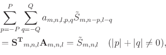
 |
(2) |
where
 denotes the transpose operator,
![$ \mathbf{S}_{m,n}=[\tilde{S}_{m,n-1}, \\
\tilde{S}_{m,n-2}, \cdots, \tilde{S}_{m,n-p}]^{\mathbf{T}}$](img18.png) denotes
the vector including the data points near
.
denotes
the vector including the data points near
.
![$ \mathbf{A}_{m,n}=[a_{m,n,1}, a_{m,n,2}, \cdots,
a_{m,n,p}]^{\mathbf{T}} $](img19.png) is the vector of coefficients in a 2D
adaptive prediction filter. Let
is the vector of coefficients in a 2D
adaptive prediction filter. Let  , Fig. 1a illustrates
how (2) works. Equation (2) denotes that
the filter predicts data point along the spatial direction rather than
the frequency direction. Therefore, an extension to the 3D
-
-
, Fig. 1a illustrates
how (2) works. Equation (2) denotes that
the filter predicts data point along the spatial direction rather than
the frequency direction. Therefore, an extension to the 3D
-
- domain is straightforward:
where
![$ l \in [1,L]$](img22.png) is the index of the data sample along the
axis.
is the index of the data sample along the
axis.
![$ p \in [-P,P]$](img23.png) and
and
![$ q \in [-Q,Q]$](img24.png) are the indices of filter
coefficients in two spatial directions,
are the indices of filter
coefficients in two spatial directions,
![$ \mathbf{A}_{m,n,l}=[a_{m,n,l,-P,-Q}, \cdots, a_{m,n,l,p,q}, \cdots,
a_{m,n,l,P,Q}]^{\mathbf{T}} $](img25.png) is the vector of 3D filter
coefficients. The adaptive prediction filter
is the vector of 3D filter
coefficients. The adaptive prediction filter
 is
defined as a space-noncausal structure and the filter size in the
spatial direction is
is
defined as a space-noncausal structure and the filter size in the
spatial direction is
 . The vector
![$ \mathbf{S}_{m,n,l}= [\tilde{S}_{m,n+P,l+Q}, \cdots,
\tilde{S}_{m,n-p,l-q}, \tilde{S}_{m,n-P,l-Q}]^{\mathbf{T}} $](img28.png) contains
the data points near
contains
the data points near
 . Let
. Let
 and
and
 , Fig. 2a demonstrates the distribution
of the vectors
, Fig. 2a demonstrates the distribution
of the vectors
 and
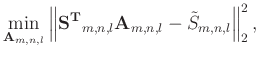
. Assuming
that the contained noise is white Gaussian noise, the filter can be
obtained by solving the minimization problem:
and
. Assuming
that the contained noise is white Gaussian noise, the filter can be
obtained by solving the minimization problem:
 |
(4) |
equation (4) describes an ill-posed problem that the number
of the unknown filter coefficients is greater than that of the known
equations. Without any regularization, the equation will lead to an
unstable solution:
 |
(5) |
where  denotes the conjugate operator.
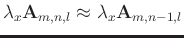
To solve the underdetermined problem (4), constraint
conditions based on local similarity/smoothness are used to stabilize
the solution of (4). Assuming that the adaptive prediction
filter at position  is similar to another one at position
 in the
-
-
domain,
in the
-
-
domain,
 can be
treated as the constraint condition on the
axis. The
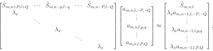
autoregression equation can be expressed as follows:
can be
treated as the constraint condition on the
axis. The
autoregression equation can be expressed as follows:
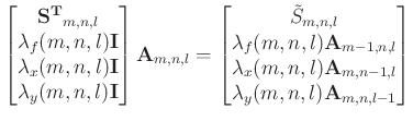
and the simplified block matrix can be written as:
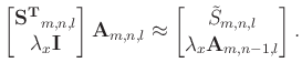 |
(7) |
Equation (7) is solvable since there are
 equations with
 unknown coefficients,
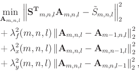
which correspond to the following minimization problem:
unknown coefficients,
which correspond to the following minimization problem:
 |
(8) |
where
 is the constant weight for the regularization term
along the
axis. In the frequency
direction, one can assume
that the SPFs change smoothly and treat the irregular perturbations as
the interference of noise. Meanwhile, the smoothness of the 3D SPFs
also exists in different spatial directions and may change at
different data point, therefore, we implemented local smoothness along
,
, and
axis as constraints to calculate the
-
-
SPF. The block matrix form is:
is the constant weight for the regularization term
along the
axis. In the frequency
direction, one can assume
that the SPFs change smoothly and treat the irregular perturbations as
the interference of noise. Meanwhile, the smoothness of the 3D SPFs
also exists in different spatial directions and may change at
different data point, therefore, we implemented local smoothness along
,
, and
axis as constraints to calculate the
-
-
SPF. The block matrix form is:
 |
(9) |
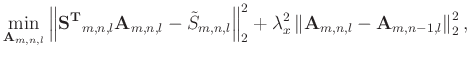
and the corresponding least-squares problem takes the
following form:
where
 ,
,
 and
and
 denotes the variable weights of regularization
terms along the frequency
axis, space
axis, and space
axis, respectively. They measure the variable similarity or closeness
between the filter
and the adjacent filters
denotes the variable weights of regularization
terms along the frequency
axis, space
axis, and space
axis, respectively. They measure the variable similarity or closeness
between the filter
and the adjacent filters
 ,
,
 , and
, and
 . Due to the prediction filter can characterize
the energy spectrum of the input data Claerbout (1976), the adaptive
filter shares analogical smoothness property with the 3D data, so the
variation of the weights may consist with the smooth version of data.
For simplicity, we select these weights with constant value,
. Due to the prediction filter can characterize
the energy spectrum of the input data Claerbout (1976), the adaptive
filter shares analogical smoothness property with the 3D data, so the
variation of the weights may consist with the smooth version of data.
For simplicity, we select these weights with constant value,
 ,
,
 and
and
 , to demonstrate the constrained
relationship. The introduced regularization terms convert the
ill-posed problem to the overdetermined inverse problem, and the
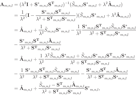
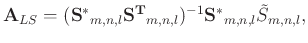
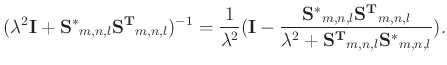
least-squares solution of (9) and (10) is:
, to demonstrate the constrained
relationship. The introduced regularization terms convert the
ill-posed problem to the overdetermined inverse problem, and the
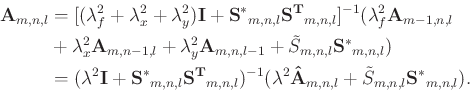
least-squares solution of (9) and (10) is:
where
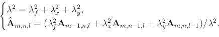 |
(12) |
The Sherman-Morrison formula is an analytic method for solving the
inverse matrix Hager (1989):
 |
(13) |
The derivation of the Sherman-Morrison formula in the complex space is
described in Appendix ![[*]](icons/crossref.png) . Elementary algebraic
simplifications lead to the analytical solution:
. Elementary algebraic
simplifications lead to the analytical solution:
Equation (14) is a recursion equation, which suggests
that the filter
recursively updates in a certain
order. The residual can be written as:
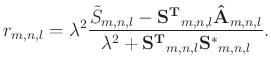 |
(15) |
Once obtaining the solution of the 3D
-
-
SPF, one can compute
the noise-free data
 with the following equation:
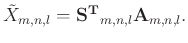 |
(16) |
The configuration of parameters
 ,
, and
,
, and
 is the basis for the proposed method. When the three
parameters are 0
, the corresponding regularization terms have no
effect on restricting the inverse problem and the result of the
-
-
SPF becomes (5). By choosing
is the basis for the proposed method. When the three
parameters are 0
, the corresponding regularization terms have no
effect on restricting the inverse problem and the result of the
-
-
SPF becomes (5). By choosing
 and removing the
axis, equation (14) is reduced
to the solution of the 2D
-
SPF. On the contrary, when the three
parameters tend to infinity, more weight is applied on regularization
terms. A large denominator in (14) indicates that the
filter cannot receive any updates to maintain its adaptive and
predictive properties. This denominator suggests that parameters
and removing the
axis, equation (14) is reduced
to the solution of the 2D
-
SPF. On the contrary, when the three
parameters tend to infinity, more weight is applied on regularization
terms. A large denominator in (14) indicates that the
filter cannot receive any updates to maintain its adaptive and
predictive properties. This denominator suggests that parameters
 and
and
 in (12) should have
the same order of magnitude as
in (12) should have
the same order of magnitude as
 , and the value of
 might be in the range of
 , which can balance
the noise suppression and signal protection. Therefore, they can
smoothly adjust the change of filters. Meanwhile, data distribution
in the frequency axis may change sharply, which is not as smooth as
those in the spatial directions; thus,
should be smaller
than
and
.
, which can balance
the noise suppression and signal protection. Therefore, they can
smoothly adjust the change of filters. Meanwhile, data distribution
in the frequency axis may change sharply, which is not as smooth as
those in the spatial directions; thus,
should be smaller
than
and
.
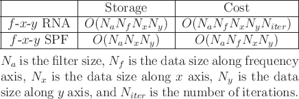
Table 1:
Cost comparison between
-
-
RNA and
-
-
SPF.
|
|


|
|---|
fig1,fig2
Figure 1. Schematic
illustration of
-
prediction filter (a) and filter processing
path (b).
|
|---|
![[png]](icons/viewmag.png) ![[scons]](icons/configure.png)
|
|---|


|
|---|
fig3,fig4
Figure 2. Schematic
illustration of
-
-
prediction filter (a) and filter
processing path in each frequency slice (b).
|
|---|
|
|
|---|
|
|
|
|
| Noniterative f-x-y streaming prediction filtering for random noise attenuation on seismic data | |
|
Next: Data processing path in
Up: Theory
Previous: Theory
2022-04-21