|
 |
 |
 | Conjugate guided gradient (CGG) method for robust inversion and its application to velocity-stack inversion |  |
![[pdf]](icons/pdf.png) |
Next: Conjugate-Guided-Gradient (CGG) method
Up: CG method for LS
Previous: CG method for LS
Instead of the  -norm solution obtained by the conventional LS method,
 -norm minimization solutions, with
  , are often tried.
Iterative inversion algorithms called IRLS
(Iteratively Reweighted Least Squares)
algorithms have been developed to solve these problems, which lie
between the least-absolute-values problem and the classical least-squares problem.
The main advantage of IRLS is that it provides an easy way to compute
the approximate -norm solution.
Among the various -norm solutions,
, are often tried.
Iterative inversion algorithms called IRLS
(Iteratively Reweighted Least Squares)
algorithms have been developed to solve these problems, which lie
between the least-absolute-values problem and the classical least-squares problem.
The main advantage of IRLS is that it provides an easy way to compute
the approximate -norm solution.
Among the various -norm solutions,
 -norm solutions are known to be more robust than -norm solutions,
being less sensitive to spiky, high-amplitude noise
Scales et al. (1988); Scales and Gersztenkorn (1987); Claerbout and Muir (1973); Taylor et al. (1979).
-norm solutions are known to be more robust than -norm solutions,
being less sensitive to spiky, high-amplitude noise
Scales et al. (1988); Scales and Gersztenkorn (1987); Claerbout and Muir (1973); Taylor et al. (1979).
The problem solved by IRLS is a minimization of the weighted residual/model
in the least-squares sense. The residual to be minimized in the weighted problem
is described as
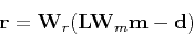 |
(5) |
where  and
and  are the weights for residual and model, respectively.
These residual and model weights are for enhancing our preference regarding
the residual and model.
They can be applied separately or together according to a given inversion goal.
In this section, for simplicity, the explanation will be limited
to the case of applying both weights together,
but the examples given in a later section will show all the cases
including the residual and the model weights separately for comparison.
Those weights can be any matrices, but diagonal matrices are often used for them
and this paper will assume all weights are diagonal matrices.
Then the gradient for the weighted least-squares becomes
are the weights for residual and model, respectively.
These residual and model weights are for enhancing our preference regarding
the residual and model.
They can be applied separately or together according to a given inversion goal.
In this section, for simplicity, the explanation will be limited
to the case of applying both weights together,
but the examples given in a later section will show all the cases
including the residual and the model weights separately for comparison.
Those weights can be any matrices, but diagonal matrices are often used for them
and this paper will assume all weights are diagonal matrices.
Then the gradient for the weighted least-squares becomes
 |
(6) |
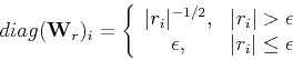
A particular choice for the residual weight is the one
that results in minimizing the -norm of the residual.
Choosing the  diagonal element of
to be a function of the component of the residual vector
as follows:
diagonal element of
to be a function of the component of the residual vector
as follows:
 |
(7) |
the -norm of the weighted residual is then
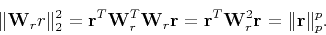 |
(8) |
Therefore, the minimization of the -norm of the weighted residual
with an weight as shown Equation (7)
can be thought as a minimization of the -norm of the residual.
This method is valid for -norms where .
When the -norm is desired, the weighting is as follows:
This weight will reduce the contribution of large residuals
and improve the fit to the data that is already well-estimated.
Thus, the -norm-based minimization is robust,
less sensitive to noise bursts in the data.
In practice the weighting operator is modified slightly to avoid dividing by zero.
For this purpose, a damping parameter  is chosen and the weighting operator is modified to be:
The choice of this parameter is related to the distribution of the residual values.
Some authors choose it as a relatively small value like
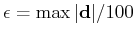 and others choose it as a value that corresponds to a small percentile of data as 2 percentile
(which is the value with 98% of the values above and 2% below).
In this paper, I used the percentile approach to decide the parameter because
it can reflect the distribution of the residual values in it
and shows more stable behavior in the experiments performed in this paper.
and others choose it as a value that corresponds to a small percentile of data as 2 percentile
(which is the value with 98% of the values above and 2% below).
In this paper, I used the percentile approach to decide the parameter because
it can reflect the distribution of the residual values in it
and shows more stable behavior in the experiments performed in this paper.
The use of the model weight is to enhance our preference regarding the model,
for example the parsimony or the smoothness of the solution.
The introduction of the model weight corresponds to applying precondition
and solving the problem
followed by
The iterative solution of this system minimizes the energy of the new model parameter

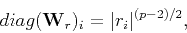
In the same vein as the residual weight, the model weight can be chosen as
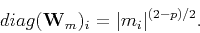 |
(9) |
Then the weighted model energy that is minimized is now
which is the -norm of the model.
When the minimum -norm model is desired, the weighting is as follows:
The IRLS method can be easily incorporated in CG algorithms by including
the weights and
such that the operator  has a postmultiplier
and a premultiplier
and the adjoint operator
has a postmultiplier
and a premultiplier
and the adjoint operator  has a premultiplier
  and
postmultiplier
and
postmultiplier  Claerbout (2004).
However, the introduction of weights that change during iterations
leads us to implement a nonlinear CG method with two nested loops.
The outer loop is for the iteration of changing weights
and the inner loop is for the iteration of the LS solution for a given weighted operator.
Even though we do not know the real residual/model vector
at the beginning of the iteration,
we can approximate the real residual/model with a residual/model
of the previous iteration step, and it will converge to
a residual/model that is very close to the real residual/model as the iteration step continues.
This method can be summarized as Algorithm 2, where
Claerbout (2004).
However, the introduction of weights that change during iterations
leads us to implement a nonlinear CG method with two nested loops.
The outer loop is for the iteration of changing weights
and the inner loop is for the iteration of the LS solution for a given weighted operator.
Even though we do not know the real residual/model vector
at the beginning of the iteration,
we can approximate the real residual/model with a residual/model
of the previous iteration step, and it will converge to
a residual/model that is very close to the real residual/model as the iteration step continues.
This method can be summarized as Algorithm 2, where  and
and  represent
functions of residual and model described in Equation (7) and Equation (9), respectively.
represent
functions of residual and model described in Equation (7) and Equation (9), respectively.
For efficiency, Algorithm 2 is often implemented not to
wait until the convergence of the inner loop
and instead implemented to finish the inner loop
after a certain number of iterations
and recomputes the weights and the corresponding residual
Darche (1989); Nichols (1994).
In order to take advantage of plane search in CG,
however, the number of the iterations of the inner loop
should be more than or equal to two.
The experiments performed for the examples of this paper have shown
almost no differences between the results of different iteration steps
of the inner loop. In this paper, therefore, the IRLS algorithm is implemented
to finish the inner loop after two iterations.
|
|
|
|
| Conjugate guided gradient (CGG) method for robust inversion and its application to velocity-stack inversion | |
|
Next: Conjugate-Guided-Gradient (CGG) method
Up: CG method for LS
Previous: CG method for LS
2011-06-26