next up previous [pdf]

Next: Computational part Up: Homework 4 Previous: Homework 4

Theoretical part

  1. Consider the elastic wave equation
    \begin{displaymath}
\rho \ddot{u}_i = C_{ijkl,j} u_{k,l} + C_{ijkl} u_{k,lj}\;
\end{displaymath} (1)

    in the case of an isotropic elasticity
    \begin{displaymath}
C_{ijkl} = \lambda \delta_{ij} \delta_{kl} +
\mu (\delta_{ik} \delta_{jl} + \delta_{il} \delta_{jk})\;.
\end{displaymath} (2)

    Using the geometric representation
    \begin{displaymath}
u_i(\mathbf{x},t) = a_i(\mathbf{x}) f\left(t-T(\mathbf{x})\right)
\end{displaymath} (3)

    and assuming the P-wave polarization in the direction of the gradient of $T$, derive the elastic P-wave amplitude transport equation and show its similarity to the corresponding equation for the case of acoustic variable-density wave propagation.
  2. Consider a 2-D common-midpoint gather $G(t,x)$, which contains a geometric event $A_0 f\left(t-T(x)\right)$ with a constant amplitude $A_0$ along a hyperbolic shape
    \begin{displaymath}
T(x) = \sqrt{t_0^2+\frac{x^2}{v^2}}\;.
\end{displaymath} (4)

    The gather gets transformed by the slant-stack (Radon transform) operator
    \begin{displaymath}
R(\tau,p) = \mathbf{D}_\tau^{1/2} \int G(\tau + p x, x) d x\;.
\end{displaymath} (5)

    where $ \mathbf{D}_\tau^{1/2}$ is a waveform-correcting half-order derivative operator.

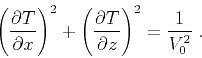
    Using the theory of geometric integration, show that $R(\tau,p)$ will contain a geometric event $A_1(p) f\left(\tau-T_1(p)\right)$. Find $T_1(p)$ and $A_1(p)$.

  3. Using the hyperbolic traveltime approximation
    \begin{displaymath}
T = \sqrt{\left(T_0-\frac{z}{V_0}\right)^2 + \frac{(x_0-x)^2}{V_0^2}}
\end{displaymath} (6)

    makes the geometric imaging analysis equivalent to analyzing wave propagation in a constant-velocity medium. In particular, we can easily verify that the traveltime satisfies the isotropic eikonal equation
    \begin{displaymath}
\left(\frac{\partial T}{\partial x}\right)^2 + \left(\frac{\partial T}{\partial z}\right)^2 = \frac{1}{V_0^2}\;.
\end{displaymath} (7)

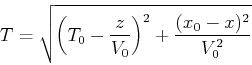
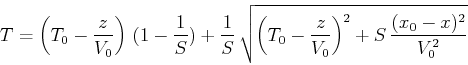
    Suppose that you switch to the more accurate shifted-hyperbola approximation

    \begin{displaymath}
T = \left(T_0-\frac{z}{V_0}\right) (1-\frac{1}{S}) + \frac{...
...\left(T_0-\frac{z}{V_0}\right)^2 + S \frac{(x_0-x)^2}{V_0^2}}
\end{displaymath} (8)

    1. How would you need to modify the eikonal equation?
    2. How would you need to modify the following expressions for the escape time and location for use in the angle-domain Kirchhoff time migration?
      $\displaystyle \hat{T}(theta)$ $\textstyle =$ $\displaystyle \frac{T_0-z/V_0}{\cos{\theta}}$ (9)
      $\displaystyle \hat{x}(theta)$ $\textstyle =$ $\displaystyle x_0 + V_0 \left(T_0-\frac{z}{V_0}\right) \tan{\theta}$ (10)


next up previous [pdf]

Next: Computational part Up: Homework 4 Previous: Homework 4

2019-11-01