|
|
|
|
GEO 365N/384S Seismic Data Processing Computational Assignment 6 |
In the first part of the assignment, we will return to processing 3D land data, the Teapot Dome dataset.
scons -cto remove (clean) previously generated files.
scons vscan.view
|
|---|
|
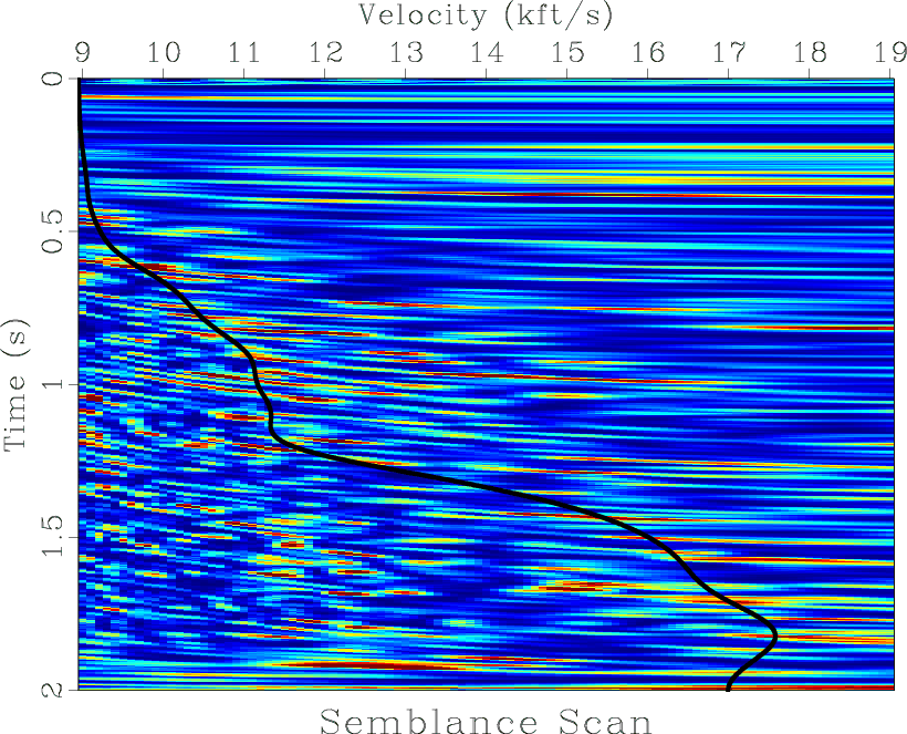
vscan
Figure 1. Semblance scan of a supergather (every 500th trace) from the Teapot Dome dataset. The curve shows the picked velocity trend. |
|
|
|
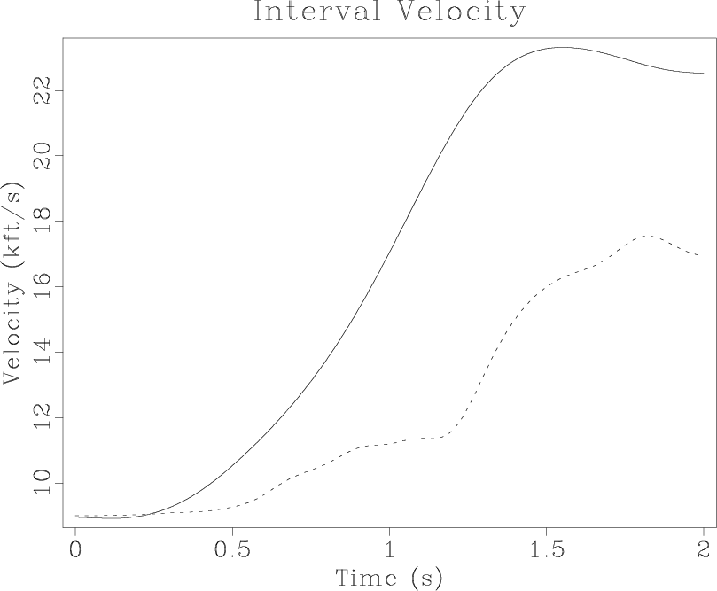
velocity
Figure 2. Interval velocity in the Teapot Dome dataset estimated by Dix inversion (regularized by smoothing). The dashed curve shows the corresponding picked RMS velocity. |
|
|---|---|
|
|
scons velocity.viewTo avoid instabilities, Dix inversion is assisted by smoothing regularization.
scons stack.view
|
|---|
|
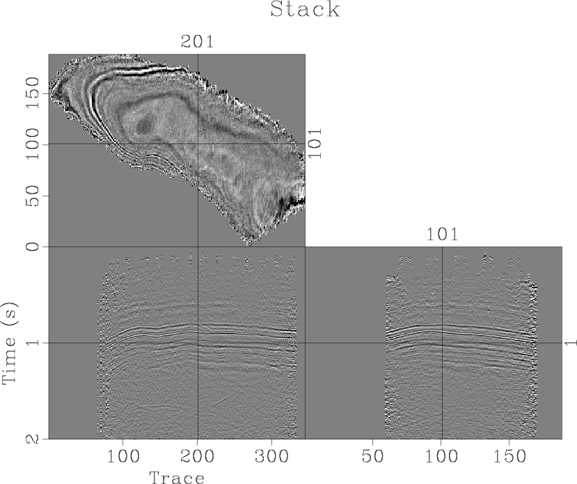
stack
Figure 3. Stack of the Teapot Dome dataset. |
|
|
scons stack2.view
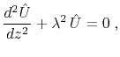
Applying the Fourier transform in time and in lateral spatial directions to the wave equation turns it into an ordinary differential equation
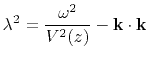
Equation (1) admits a depth-stepping solution
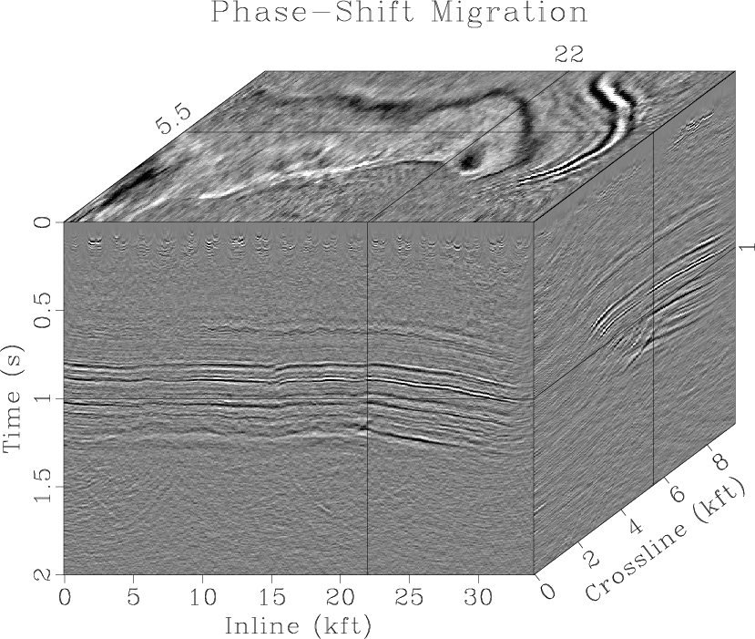
To generate a 3D phase-shift migration of the stack in Figure 3, run
scons image.viewThe computation proceeds in the vertical time coordinates, with the result displayed on the same grid as the input. To compare the data before and after migration, run
sfpen Fig/stack2.vpl Fig/image.vplDo you observe notable differences?
|
|---|
|
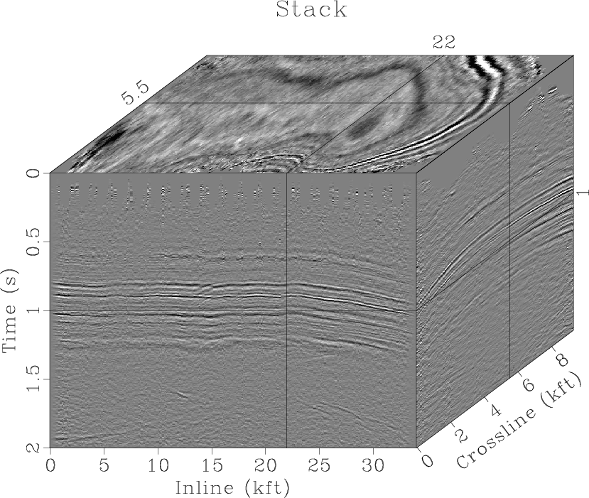
stack2,image
Figure 4. Portion of the rotated Teapot Dome stack (a) and its migration by the phase-shift method displayed in vertical time (b). |
|
|

instead of

Which sign (plus or minus) should be used in equation (2) for post-stack migration?

|
|---|
|
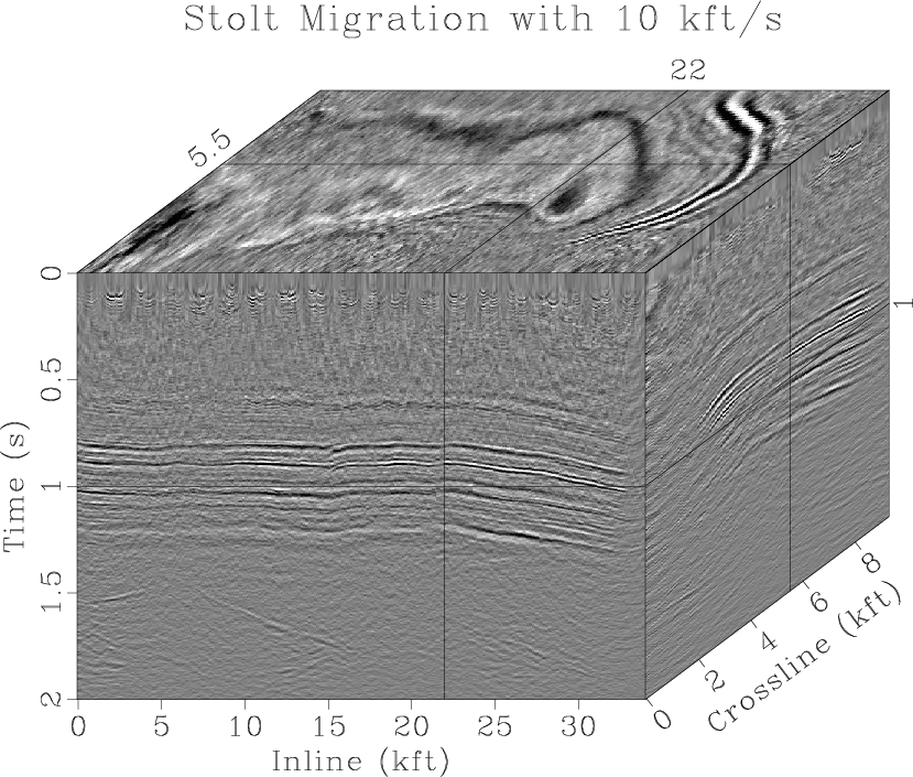
mig10,migst
Figure 5. Portion of the rotated Teapot Dome stack migrated using Stolt migration. (a) Using a constant velocity of 10 kft/s. (b) Using the Stolt stretch method. |
|
|
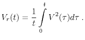
Figure 5a shows the result of Stolt migration without stretch and using velocity of 10 kft/s. Figure 5b is the result of Stolt migration using the stretch approach. To display these figures on your screen, run
scons mig10.view migst.view
You can compare the CPU time of different methods experimentally by running scons TIMER=y instead of scons.
sfpen Fig/image.vpl Fig/migst.vpl
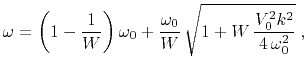
Try improving the match by modifying the value of the Stolt-stretch parameter ![]() from the value of
from the value of ![]() . You can find a better value by experimentation or by using the appropriate theory (Fomel and Vaillant, 2001).
. You can find a better value by experimentation or by using the appropriate theory (Fomel and Vaillant, 2001).
from rsf.proj import *

# Download Teapot Dome field data
Fetch('npr3_gathers.sgy','teapot',
      server='http://s3.amazonaws.com',top='')
#Fetch('npr3_gathers.sgy','TeapotDome3D',
#      top='/home/p1/seismic_datasets/SeismicProcessingClass',
#      server='local')

# Convert from SEGY to RSF
Flow('traces header header.asc','npr3_gathers.sgy',
     '''
     segyread tfile=${TARGETS[1]} hfile=${TARGETS[2]} |
     window max1=2
     ''')

# Seismic data corresponds to trid=1
Flow('trid','header','headermath output=trid | mask min=1 max=1')

Flow('tcmp','header trid','headerwindow mask=${SOURCES[1]}')
Flow('cmps','traces trid','headerwindow mask=${SOURCES[1]}')

# Extract offset, convert from ft to kft
Flow('offset','tcmp',
     '''
     headermath output=offset |
     dd type=float | scale dscale=0.001
     ''')

# Velocity analysis using a supergather
#######################################

# take every 500th trace
Flow('subcmps','cmps','window j2=500')
Flow('suboffset','offset','window j2=500')

Flow('vscan','subcmps suboffset',
     '''
     vscan offset=${SOURCES[1]} half=n semblance=y
     v0=9 nv=101 dv=0.1
     ''')
Plot('vscan',
     '''
     grey color=j allpos=y title="Semblance Scan"
     unit2=kft/s
     ''')

Flow('vpick','vscan',
     '''
     mutter inner=y x0=9 half=n t0=0.5 v0=3 |
     scale axis=2 | pick rect1=50
     ''')
Plot('vpick',
     '''
     graph yreverse=y transp=y plotcol=7 plotfat=7
     pad=n min2=9 max2=19 wantaxis=n wanttitle=n
     ''')

Result('vscan','vscan vpick','Overlay')

# Dix conversion to interval velocity
Flow('semb','vscan vpick','slice pick=${SOURCES[1]}')
Flow('vdix','vpick semb','dix weight=${SOURCES[1]} rect1=50')

Result('velocity','vdix vpick',
       '''
       cat axis=2 ${SOURCES[1]} |
       graph dash=0,1 title="Interval Velocity" unit2=kft/s
       ''')

# NMO and stack
###############

Flow('binorder','tcmp','headermath output="345*xline+iline" ')
Flow('tcmp2','tcmp binorder','headersort head=${SOURCES[1]}')
Flow('cmps2','cmps binorder tcmp2',
     '''
     headersort head=${SOURCES[1]} |
     intbin3 head=${SOURCES[2]} xkey=-1 yk=iline zk=xline
     ''')
Flow('offset2 mask','offset binorder tcmp2',
     '''
     headersort head=${SOURCES[1]} |
     intbin3 head=${SOURCES[2]} xkey=-1 yk=iline zk=xline
     mask=${TARGETS[1]}
     ''')

Flow('vpick3','vpick',
    '''
    spray axis=2 n=1 | spray axis=3 n=345 | spray axis=4 n=188
    ''')
Flow('mask3','mask','spray axis=1 n=1')

Flow('nmo','cmps2 offset2 mask3 vpick3',
     '''
     nmo offset=${SOURCES[1]} half=n
     mask=${SOURCES[2]} velocity=${SOURCES[3]}
     ''',split=[4,'omp'])

Flow('stack','nmo','stack')

Result('stack',
       '''
       byte gainpanel=all |
       grey3 frame1=500 frame2=200 frame3=100 title=Stack
       ''')

# Rotate and window

import math
az = 70*math.pi/180 # azimuth angle

nx=345
ny=188
nxy=nx*ny

Flow('x','stack',
     '''
     window n1=1 |
     math output="%g+(%g)*x1+(%g)*x2"
     ''' % (nx*0.5, math.cos(az),math.sin(az)))
Flow('y','x',
     '''
     math output="%g+(%g)*x1+(%g)*x2"
     ''' % (ny*0.5,-math.sin(az),math.cos(az)))

Flow('xy','x y',
     '''
     cat axis=3 ${SOURCES[1]} | put n1=%d n2=1 |
     window | transp
     ''' % nxy)

Flow('stack2','stack xy',
     '''
     put n2=%d n3=1 |
     transp memsize=5000 |
     bin xkey=0 ykey=1 head=${SOURCES[1]}
     nx=85 x0=295 dx=1 ny=310 y0=-200 dy=1 interp=2 |
     costaper nw2=10 nw3=10 |
     transp plane=13 memsize=5000 |
     put o2=0 d2=0.11 o3=0 d3=0.11
     unit2=kft label2=Inline unit3=kft label3=Crossline
     ''' % nxy)

Result('stack2',
       '''
       byte gainpanel=all |
       grey3 frame1=500 frame2=200 frame3=50
       title=Stack point1=0.7 point2=0.7 flat=n
       ''')

# Fourier transform in space

Flow('cosft','stack2','cosft sign2=1 sign3=1')

# Phase-shift migration
#######################

Flow('gazdag','cosft vdix',
     'gazdag velocity=${SOURCES[1]} verb=y',
     split=[3,'omp',[0]])

Flow('image','gazdag','cosft sign2=-1 sign3=-1')

Result('image',
       '''
       byte gainpanel=all |
       grey3 frame1=500 frame2=200 frame3=50
       title="Phase-Shift Migration" point1=0.7 point2=0.7 flat=n
       ''')

# Stolt migration with 10 kft/s
Flow('cosft3','cosft','cosft sign1=1')

Flow('map10','cosft3',
     'math output="sqrt(x1*x1+25*(x2*x2+x3*x3))" ')

Flow('stolt10','cosft3 map10',
     'iwarp warp=${SOURCES[1]} inv=n',split=[3,'omp'])

Flow('mig10','stolt10','cosft sign1=-1 sign2=-1 sign3=-1')

Result('mig10',
       '''
       byte gainpanel=all |
       grey3 frame1=500 frame2=200 frame3=50
       title="Stolt Migration with 10 kft/s"
       point1=0.7 point2=0.7 flat=n
       ''')

# Apply Stolt stretch
Flow('cosftst','cosft vdix',
     'stoltstretch velocity=${SOURCES[1]} vel=10 | cosft sign1=1')

# Stolt stretch parameter
#########################
st=1.5 # !!! MODIFY ME !!!

Flow('mapst','cosft3',
     '''
     math output="(1-1/%g)*x1+sqrt(x1*x1+%g*(x2*x2+x3*x3))/%g"
     ''' % (st,st*25,st))

Flow('stoltst','cosftst mapst',
     'iwarp warp=${SOURCES[1]} inv=n',split=[3,'omp'])

Flow('migst','stoltst vdix',
     '''
     cosft sign1=-1 sign2=-1 sign3=-1 |
     stoltstretch velocity=${SOURCES[1]} vel=10 inv=y
     ''')

Result('migst',
       '''
       byte gainpanel=all |
       grey3 frame1=500 frame2=200 frame3=50
       title="Stolt Migration with Stolt Stretch"
       point1=0.7 point2=0.7 flat=n
       ''')

End()
|
|
|
|
|
GEO 365N/384S Seismic Data Processing Computational Assignment 6 |