GEO 365N/384S Seismic Data Processing Computational Assignment 3

NMO Velocity Analysis with 3D Land Data

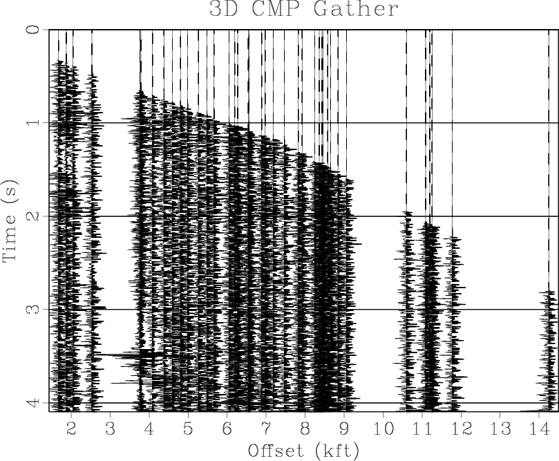
In the final section, we will apply NMO-based velocity analysis to a CMP gather from the Teapot Dome 3D land dataset.

1. Change directory to hw3/nmo3d.
2. Run

   scons -c
   

   to remove (clean) previously generated files.
3. The input data for this exercise have been preprocessed to prepare them for prestack migration and velocity analysis. We will start by selecting a CMP gather at in-line 200 and cross-line 100 (Figure 14.) You can refer to the acquisition geometry analysis from Computational Assignment 2 to locate this gather inside the survey.

   

   cmp3
   Figure 14. Selected CMP gather from the Teapot Dome dataset.

   

   
   

   To display the gather in a wiggle plot, run

   scons cmp3.view
   

4. Despite the preprocessing, the data remain noisy. To examine how the NMO correction may affect seismic events, we can apply it first with an ensemble of constant velocities (Figure 15.)

   To display the result, run

   scons nmos.view
   

   What is the apparent velocity of the event arriving around 1 second?

   

   

   nmos
   Figure 15. Constant-velocity NMO corrections applied to the Teapot Dome CMP gather.

   

   
   

5. Similarly to the 2D data, we can analyze velocities using semblance scans. To pick velocities, we will use, for a change, manual interactive picking (Figure 16.)

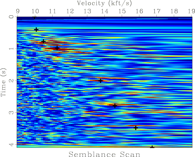
   To perform manual picking, uncomment the lines in the SConstruct file, which involve the sfipick program. Then run

   scons picks3.view
   

   to perform your own manual picking.

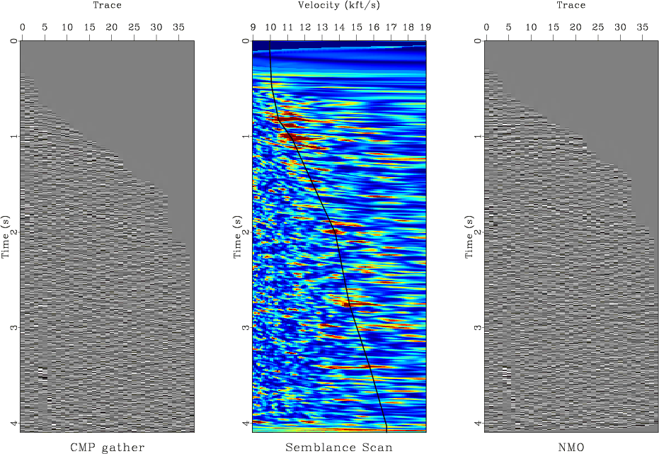
   Run

   scons nmo3.view
   

   to display the NMO correction result (Figure 17.)

   

   picks
   Figure 16. Semblance scan with interactive picks.

   

   
   

   

   nmo3
   Figure 17. Velocity analysis using manual picking and NMO applied to the Teapot Dome CMP gather.

   

   
   

6. Your final task: choose a different CMP gather (possibly the one with the highest CMP fold) and repeat the analysis.

from rsf.proj import *

# Download Teapot Dome field data
#Fetch('npr3_gathers.sgy','teapot',
#      server='http://s3.amazonaws.com',top='')
Fetch('npr3_gathers.sgy','TeapotDome3D',
      top='/home/p1/seismic_datasets/SeismicProcessingClass',
      server='local')

# Convert from SEGY to RSF
Flow('traces header header.asc','npr3_gathers.sgy',
     'segyread tfile=${TARGETS[1]} hfile=${TARGETS[2]}')

# Seismic data corresponds to trid=1
Flow('trid','header','headermath output=trid | mask min=1 max=1')

################################################################
# Extract CMP gather at xline=100 iline=200 !!! MODIFY BELOW !!! 
################################################################
Flow('xline','header',
     'headermath output=xline | mask min=100 max=100')
Flow('iline','header',
     'headermath output=iline | mask min=200 max=200')
Flow('maskcmp','trid xline iline','mul ${SOURCES[1:3]}')

Flow('tcmp','header maskcmp','headerwindow mask=${SOURCES[1]}')

# Extract offset, convert from ft to kft
Flow('offset0','tcmp',
     '''
     headermath output=offset | 
     dd type=float | scale dscale=0.001
     ''')
Flow('offset','offset0','headersort head=$SOURCE')
Flow('cmp','traces maskcmp offset0',
     '''
     headerwindow mask=${SOURCES[1]} | 
     headersort head=${SOURCES[2]} | 
     bandpass flo=5
     ''')

Result('cmp3','cmp offset',
       '''
       wiggle poly=y yreverse=y transp=y xpos=${SOURCES[1]} 
       label2=Offset unit2=kft title="3D CMP Gather" 
       ''')

# Scan different NMO velocities
nmos = []
for v in range(10,20):
    nmo = 'nmo%d' % v
    vel = 'vel%d' % v
    Flow(vel,'cmp','spike n1=2049 mag=%d' % v)
    Flow(nmo,['cmp','offset',vel],
         'nmo half=n offset=${SOURCES[1]} velocity=${SOURCES[2]}')
    nmos.append(nmo)
Result('nmos',nmos,
       '''
       merge axis=2 ${SOURCES[1:%d]} | window min1=0.5 max1=2.5 | 
       grey title="NMO Scan from 10 kft/s to 19 kft/s" wantaxis2=n
       ''' % len(nmos))

Flow('vscan','cmp offset',
     '''
     vscan half=n semblance=y v0=9 nv=101 dv=0.1 
     offset=${SOURCES[1]} nb=4
     ''')

Plot('vscan',
     'grey color=j allpos=y title="Semblance Scan" unit2=kft/s')

# Interactive picking

# !!! UNCOMMENT NEXT TWO LINES !!!
#Flow('picks.txt','vscan',
#     'ipick color=j allpos=y wanttitle=n unit2=kft/s')

Flow('picks','picks.txt',
     '''
     wc -l | 
     sed 's/^/in=$SOURCE data_format=ascii_float n1=3 n2=/' |
     dd form=native | window n1=2
     ''')

Plot('picks',
     '''
     dd type=complex | window | 
     graph symbol=+ symbolsz=8 yreverse=y transp=y wanttitle=n
     plotcol=7 plotfat=7 pad=n min2=9 max2=19 wantaxis=n 
     ''')

Result('picks','vscan picks','Overlay')

Flow('vpick','picks vscan',
     'transp | linear pattern=${SOURCES[1]} rect=5 sort=y')

Plot('vpick',
     '''
     graph yreverse=y transp=y plotcol=7 plotfat=7 
     pad=n min2=9 max2=19 wantaxis=n wanttitle=n
     ''')

Plot('vscan3','vscan vpick','Overlay')

# Apply NMO

Flow('nmo','cmp offset vpick',
     'nmo half=n offset=${SOURCES[1]} velocity=${SOURCES[2]}')

Plot('cmp','grey title="CMP gather" ')
Plot('nmo','grey title=NMO')

Result('nmo3','cmp vscan3 nmo','SideBySideAniso',
       vppen='txscale=1.5')

End()

GEO 365N/384S Seismic Data Processing Computational Assignment 3