|
|
|
|
Homework 1 |
|
byte
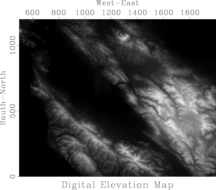
Figure 1. Digital elevation map of the San Francisco Bay area. |
|
|---|---|
|
|
Figure 1 shows a digital elevation map of the San Francisco Bay area. Start by reproducing this figure on your screen.
hw1/dem
scons byte.view
sfin byte.rsfto check the data size and format.
sfattr < byte.rsfto check data attributes. What is the maximum and minimum value? What is the mean value? For an explanation of different attributes, run sfattr without input.
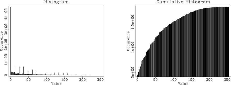
Each image has a certain distribution of values (a histogram). The histogram for the west Austin elevation map is shown in Figure 2. Notice the digitization artifacts. When different values in a histogram are not uniformly distributed, the image can have a low contrast. One way of improving the contrast is histogram equalization.
|
|---|
|
hist
Figure 2. Histogram (left) and cumulative histogram (right) of the digital elevation data. |
|
|
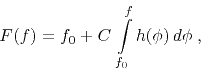
Let ![]() be the original image. The equalized image will be
be the original image. The equalized image will be
![]() . Let
. Let ![]() be the histogram (probability distribution) of
the original image values. Let
be the histogram (probability distribution) of
the original image values. Let ![]() be the histogram of the modified
image. The mapping of probabilities suggests
be the histogram of the modified
image. The mapping of probabilities suggests
The algorithm for histogram equalization consists of the following three steps:
Your task:
scons hist.viewto display the figure on your screen.
from rsf.proj import *

# Download data
Fetch('bay.h','bay')

# Convert to byte form
Flow('byte','bay.h',
     '''
     dd form=native |
     window f2=500 n2=1500 |
     byte pclip=100 allpos=y
     ''')

# Display
Result('byte',
       '''
       grey yreverse=n label1=South-North label2=West-East
       title="Digital Elevation Map" screenratio=0.8
       ''')

# Histogram
Flow('hist','byte',
     '''
     dd type=float |
     histogram n1=256 o1=0 d1=1 |
     dd type=float
     ''')
Plot('hist',
     'bargraph label1=Value label2=Occurence title=Histogram')

# Cumulative histogram
Flow('cumu','hist','causint')

Plot('cumu',
       '''
       bargraph label1=Value label2=Occurence
       title="Cumulative Histogram"
       ''')

Result('hist','hist cumu','SideBySideIso')

# ADD HISTOGRAM EQUALIZATION

End()
|
|
|
|
|
Homework 1 |