|
|
|
|
Multidimensional autoregression |
|
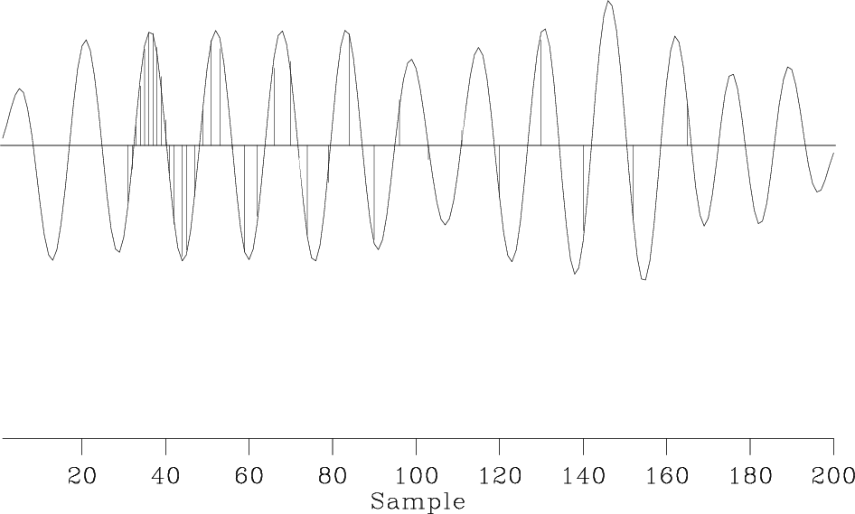
subsine3
Figure 26. Interpolating with a three-term filter. The interpolated signal is fairly monofrequency. |
|
|---|---|
|
|
|
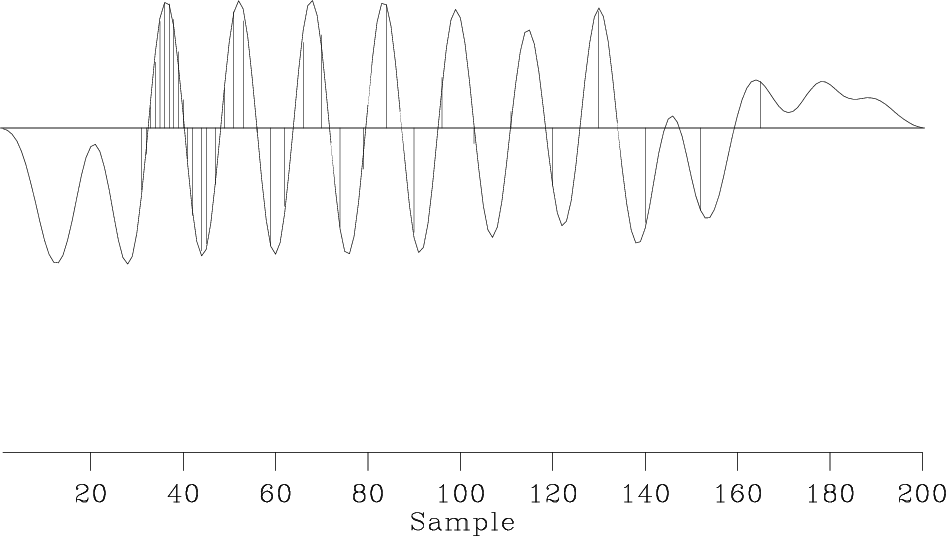
subsine5
Figure 27. Interpolating with a five term filter. |
|
|---|---|
|
|
Comparing Figures
![]() and
and
![]() to
Figures 26 and 27
we conclude that by finding and imposing
the prediction-error filter
while finding the model space,
we have interpolated beyond aliasing in data space.
to
Figures 26 and 27
we conclude that by finding and imposing
the prediction-error filter
while finding the model space,
we have interpolated beyond aliasing in data space.
| Sometimes PEFs enable us to interpolate beyond aliasing. |
|
|
|
|
Multidimensional autoregression |