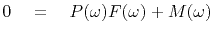
 |
 |
 |
 | Multidimensional autoregression |  |
![[pdf]](icons/pdf.png) |
Next: TIME-SERIES AUTOREGRESSION
Up: Multidimensional autoregression
Previous: Time domain versus frequency
Here we devise a simple mathematical model
for deep water bottom multiple reflections.![[*]](icons/footnote.png) There are two unknown waveforms,
the source waveform
There are two unknown waveforms,
the source waveform
 and the ocean-floor reflection
 .
The water-bottom primary reflection
.
The water-bottom primary reflection
 is the convolution of the source waveform
with the water-bottom response; so
is the convolution of the source waveform
with the water-bottom response; so
 .
The first multiple reflection
.
The first multiple reflection
 sees the same source waveform,
the ocean floor, a minus one for the free surface, and the ocean floor again.
Thus the observations
and
as functions of the physical parameters are
sees the same source waveform,
the ocean floor, a minus one for the free surface, and the ocean floor again.
Thus the observations
and
as functions of the physical parameters are
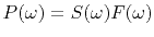
Algebraically the solutions of equations
(1) and
(2) are
These solutions can be computed in the Fourier domain
by simple division.
The difficulty is that the divisors in
equations (3) and (4)
can be zero, or small.
This difficulty can be attacked by use of a positive number  to stabilize it.
For example, multiply equation (3) on top and bottom
by
to stabilize it.
For example, multiply equation (3) on top and bottom
by
 and add
 to the denominator.
This gives
to the denominator.
This gives
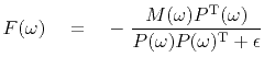 |
(5) |
where
 is the complex conjugate of
.
Although the
stabilization seems nice,
it apparently produces a nonphysical model.
For
large or small, the time-domain response
could turn out to be of much greater duration than is physically reasonable.
This should not happen with perfect data, but in real life,
data always has a limited spectral band of good quality.
is the complex conjugate of
.
Although the
stabilization seems nice,
it apparently produces a nonphysical model.
For
large or small, the time-domain response
could turn out to be of much greater duration than is physically reasonable.
This should not happen with perfect data, but in real life,
data always has a limited spectral band of good quality.
Functions that are rough in the frequency domain will be long in
the time domain.
This suggests making a short function in the time domain
by local smoothing in the frequency domain.
Let the notation
 denote smoothing by local averaging.
Thus,
to specify filters whose time duration is not unreasonably long,
we can revise equation (5) to
denote smoothing by local averaging.
Thus,
to specify filters whose time duration is not unreasonably long,
we can revise equation (5) to
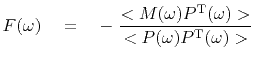 |
(6) |
where
instead of deciding a size for
we need to decide how much smoothing.
I find that smoothing has a simpler physical interpretation than choosing
.
The goal of finding the filters
and
is to
best model the multiple reflections so that they can
be subtracted from the data,
and thus enable us to see what primary reflections
have been hidden by the multiples.
These frequency-duration difficulties do not arise in a time-domain formulation.
Unlike in the frequency domain,
in the time domain it is easy and natural
to limit the duration and location
of the nonzero time range of
and
.
First express
(3) as
 |
(7) |
To imagine equation (7)
as a fitting goal in the time domain,
instead of scalar functions of  ,
think of vectors with components as a function of time.
Thus
,
think of vectors with components as a function of time.
Thus  is a column vector
containing the unknown sea-floor filter,
is a column vector
containing the unknown sea-floor filter,
 contains the ``multiple'' portion of a seismogram,
and
contains the ``multiple'' portion of a seismogram,
and  is a matrix of down-shifted columns,
each column being the ``primary''.
is a matrix of down-shifted columns,
each column being the ``primary''.
![$\displaystyle \bold 0 \quad\approx\quad \bold r \eq \left[ \begin{array}{c} r_1...
...ay}{c} m_1 \ m_2 \ m_3 \ m_4 \ m_5 \ m_6 \ m_7 \ m_8 \end{array} \right]$](img29.png) |
(8) |
|
|
|
|
| Multidimensional autoregression | |
|
Next: TIME-SERIES AUTOREGRESSION
Up: Multidimensional autoregression
Previous: Time domain versus frequency
2013-07-26