Model fitting by least squares

Formal path to the low-cut filter

This book defines many geophysical estimation applications. Many applications amount to fitting two goals. The first goal is a data-fitting goal, the goal that the model should imply some observed data. The second goal is that the model be not too big nor too wiggly. We state these goals as two residuals, each of which is ideally zero. A very simple data fitting goal would be that the model $m$ equals the data $d$, thus the difference should vanish, say $0\approx m- d$. A more interesting goal is that the model should match the data especially at high frequencies but not necessarily at low frequencies.

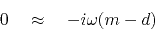$$0 \quad\approx\quad -i\omega(m - d)$$ (9)

A danger of this goal is that the model could have a zero-frequency component of infinite magnitude as well as large amplitudes for low frequencies. To suppress such bad behavior we need the second goal, a model residual to be minimized. We need a small number $\epsilon$. The model goal is:

$$0 \quad\approx\quad \epsilon \ m$$ (10)

To see the consequence of these two goals, we add the squares of the residuals:

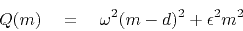$$Q(m) \eq \omega^2 (m-d)^2 + \epsilon^2 m^2$$ (11)

and then, we minimize $Q(m)$ by setting its derivative to zero:

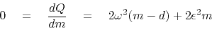$$0\eq {dQ\over dm} \eq 2 \omega^2 (m-d) + 2\epsilon^2 m$$ (12)

or

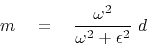$$m \eq {\omega^2 \over \omega^2+ \epsilon^2}\ d$$ (13)

Let us rename $\epsilon$ to give it physical units of frequency $\omega_0 = \epsilon$. Our expression says says $m$ matches $d$ except for low frequencies $\vert m\vert <\vert\omega_0\vert$ where it tends to zero. Now we recognize we have a low-cut filter with ``cut-off frequency'' $\omega_0$.

Model fitting by least squares