Model fitting by least squares

Standard methods

The conjugate-direction method is really a family of methods. Mathematically, where there are $n$ unknowns, these algorithms all converge to the answer in $n$ (or fewer) steps. The various methods differ in numerical accuracy, treatment of underdetermined systems, accuracy in treating ill-conditioned systems, space requirements, and numbers of dot products. Technically, the method of CD used in the cgstep module is not the conjugate-gradient method itself, but is equivalent to it. This method is more properly called the conjugate-direction method with a memory of one step. I chose this method for its clarity and flexibility. If you would like a free introduction and summary of conjugate-gradient methods, I particularly recommend An Introduction to Conjugate Gradient Method Without Agonizing Pain by Jonathon Shewchuk, which you can downloadhttp://www.cs.cmu.edu/afs/cs/project/quake/public/papers/painless-conjugate-gradient.ps.

I suggest you skip over the remainder of this section and return after you have seen many examples and have developed some expertise, and have some technical problems.

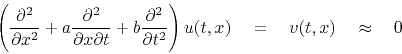
The conjugate-gradient method was introduced by Hestenes and Stiefel in 1952. To read the standard literature and relate it to this book, you should first realize that when I write fitting goals like

$$0 \approx \bold W( \bold F \bold m - \bold d )$$ (112)

$$0 \approx \bold A \bold m,$$ (113)

they are equivalent to minimizing the quadratic form:

$$\bold m: \quad\quad \min_{\bold m} Q(\bold m) \eq ( \bold m\... ...F \bold m - \bold d) \ +\ \bold m\T\,\bold A\T\,\bold A\bold m$$ (114)

The optimization theory (OT) literature starts from a minimization of

$$\bold x: \quad\quad \min_{\bold x} Q(\bold x) \eq \bold x\T\,\bold H \bold x - \bold b\T\,\bold x$$ (115)

To relate equation (114) to (115) we expand the parentheses in (114) and abandon the constant term $\bold d\T\,\bold d$. Then gather the quadratic term in $\bold m$ and the linear term in $\bold m$. There are two terms linear in $\bold m$ that are transposes of each other. They are scalars so they are equal. Thus, to invoke ``standard methods,'' you take your problem-formulation operators $\bold F$, $\bold W$, $\bold A$ and create two subroutines that apply:

$$\bold H = \bold F\T\,\bold W\T\,\bold W\bold F + \bold A\T\,\bold A$$ (116)

$$\bold b\T = 2(\bold F\T\,\bold W\T\,\bold W\bold d)\T$$ (117)

The operators $\bold H$ and $\bold b\T$ operate on model space. Standard procedures do not require their adjoints because $\bold H$ is its own adjoint and $\bold b\T$ reduces model space to a scalar. You can see that computing $\bold H$ and $\bold b\T$ requires one temporary space the size of data space (whereas cgstep requires two).

When people have trouble with conjugate gradients or conjugate directions, I always refer them to the Paige and Saunders algorithm LSQR. Methods that form $\bold H$ explicitly or implicitly (including both the standard literature and the book3 method) square the condition number, that is, they are twice as susceptible to rounding error as is LSQR. The Paige and Saunders method is reviewed by Nolet in a geophysical context.

EXERCISES:

1. It is possible to reject two dips with the operator:
   

   $$(\partial_x + p_1 \partial_t)(\partial_x + p_2 \partial_t)$$ (118)

   
   
   This is equivalent to:
   

   $$\left( \frac{\partial^2}{\partial x^2} + a \frac{\partial^2}... ...\partial t^2} \right) u(t,x) \eq v(t,x) \quad \approx \quad 0$$ (119)

   
   
   where $u$ is the input signal, and $v$ is the output signal. Show how to solve for $a$ and $b$ by minimizing the energy in $v$.

2. Given $a$ and $b$ from the previous exercise, what are $p_1$ and $p_2$?

3. Reduce $\bold d = \bold F \bold m$ to the special case of one data point and two model points like this:
   

   $$d \quad =\quad \left[ \begin{array}{cc} 2 & 1 \end{array}\right] \left[ \begin{array}{c} m_1 \\ m_2 \end{array}\right]$$ (120)

   
   
   What is the null space?

4. In 1695, 150 years before Lord Kelvin's absolute temperature scale, 120 years before Sadi Carnot's PhD. thesis, 40 years before Anders Celsius, and 20 years before Gabriel Fahrenheit, the French physicist Guillaume Amontons, deaf since birth, took a mercury manometer (pressure gauge) and sealed it inside a glass pipe (a constant volume of air). He heated it to the boiling point of water at 100$^\circ$C. As he lowered the temperature to freezing at 0$^\circ$C, he observed the pressure dropped by 25% . He could not drop the temperature any further, but he supposed that if he could drop it further by a factor of three, the pressure would drop to zero (the lowest possible pressure), and the temperature would have been the lowest possible temperature. Had he lived after Anders Celsius, he might have calculated this temperature to be $-300^\circ$C (Celsius). Absolute zero is now known to be $-273^\circ$C.

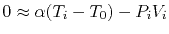   It is your job to be Amontons' lab assistant. You make your i-th measurement of temperature $T_i$ with Issac Newton's thermometer; and you measure pressure $P_i$ and volume $V_i$ in the metric system. Amontons needs you to fit his data with the regression $0 \approx \alpha (T_i - T_0 ) - P_i V_i$ and calculate the temperature shift $T_0$ that Newton should have made when he defined his temperature scale. Do not solve this problem! Instead, cast it in the form of equation (), identifying the data $d$ and the two column vectors $f_1$ and $f_2$ that are the fitting functions. Relate the model parameters $x_1$ and $x_2$ to the physical parameters $\alpha$ and $T_0$ . Suppose you make ALL your measurements at room temperature, can you find $T_0$ ? Why or why not?

5. One way to remove a mean value $m$ from signal $s(t)= \bold s$ is with the fitting goal $\bold 0 \approx \bold s - m$. What operator matrix is involved?

6. What linear operator subroutine from Chapter can be used for finding the mean?

7. How many CD iterations should be required to get the exact mean value?

8. Write a mathematical expression for finding the mean by the CG method.

Model fitting by least squares