The helical coordinate

Causality in three dimensions

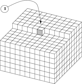
The top plane in Figure 8 is the 2-D filter seen in equation (9). Geometrically, the 3-dimensional generalization of a helix, Figure 8 shows a causal filter in three dimensions. Think of the little cubes as packed with the string of the causal 1-D function. Under the ``1'' is packed with string, but none above it. Behind the ``1'' is packed with string, but none in front of it. The top plane can be visualized as the area around the end of the 1-D string. Above the top plane are zero-valued anticausal filter coefficients.

This 3-D cube is like the usual Fortran packing of a 3-D array with one confusing difference. The starting location where the ``1'' is located is not at the Fortran (1,1,1) location. Details of indexing are essential, but complicated, and found near the end of this chapter.

3dpef Figure 8. A 3-D causal filter at the starting end of a 3-D helix.

The ``1'' that defines the end of the 1-dimensional filter becomes in 3-D a point of central symmetry. Every point inside a 3-D filter has a mate opposite the ``1'' that is outside the filter. Altogether they fill the whole space leaving no holes. From this you may deduce that the ``1'' must lie on the side of a face as shown in Figure 8. It cannot lie on the corner of a cube. It cannot be at the Fortran of f(1,1,1). If it were there, the filter points inside with their mirror points outside would not full the entire space. It could not represent all possible 3-D autocorrelation functions.

The helical coordinate