Basic operators and adjoints

The basic low-cut filter

Many geophysical measurements contain very low-frequency noise called ``drift.'' For example, it might take some months to survey the depth of a lake. Meanwhile, rainfall or evaporation could change the lake level so that new survey lines become inconsistent with old ones. Likewise, gravimeters are sensitive to atmospheric pressure, which changes with the weather. A magnetic survey of an archeological site would need to contend with the fact that the Earth's main magnetic field is changing randomly through time while the survey is being done. Such noise is sometimes called ``secular noise.''

The simplest way to eliminate low-frequency noise is to take a time derivative. A disadvantage is that the derivative changes the waveform from a pulse to a doublet (finite difference). Here we examine the most basic low-cut filter. It preserves the waveform at high frequencies, it has an adjustable parameter for choosing the bandwidth of the low cut, and it is causal (uses the past but not the future).

We make a causal low-cut filter (high-pass filter) by two stages that can be done in either order.

1. Apply a time derivative, actually a finite difference, convolving the data with $(1,-1)$.
2. Do a leaky integration dividing by $1-\rho Z$ where numerically, $\rho$ is slightly less than unity.

The convolution with $(1,-1)$ ensures the zero frequency is removed. The leaky integration almost undoes the differentiation but cannot restore the zero frequency. Adjusting the numerical value of $\rho$ has interesting effects in the time domain and in the frequency domain. Convolving the finite difference $(1,-1)$ with the leaky integration $(1, \rho, \rho^2, \rho^3, \rho^4, \cdots)$ gives the result:

$$( 1, \rho, \rho^2, \rho^3, \rho^4, \cdots)$$

$$- (0, 1, \rho, \rho^2, \rho^3, \cdots).$$

Rearranging, it becomes:

$$( 1, 0, 0, 0, 0, \cdots) +$$

$$(\rho-1) (0, 1, \rho, \rho^2, \rho^3, \cdots).$$

Because $\rho$ is a tiny bit less than one, $(1-\rho)$ is a small number. Thus, our filter is an impulse followed by the negative of a weak decaying exponential $\rho^t$. If you prefer a time-symmetric (phaseless) filter, you could follow this one by its time reverse.

Roughly speaking, the cut-off frequency of the filter corresponds to matching one wavelength to the exponential decay time. More formally, the Fourier domain representation of this filter is $H(Z) = (1-Z)/(1-\rho Z)$, where $Z$ is the unit-delay operator is $Z=e^{i\omega\Delta t}$, and where $\omega$ is the frequency. The spectral response of the filter is $\vert H(\omega)\vert$. Were we to plot this function, we would see it is nearly 1 everywhere except in a small region near $\omega=0$ where it becomes tiny. Figure 6 compares a low-cut filter to a finite difference.

galocut
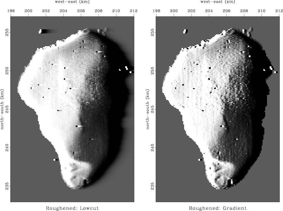
Figure 6. The depth of the Sea of Galilee after roughening. On the left, the smoothing is done by low-cut filtering on the horizontal axis. On the right it is a finite difference. We see which is which because of a few scattered impulses (navigation failure) outside the lake. Both results solve the problem of Figure 3 that it is too smooth to see interesting features.

Basic operators and adjoints