|
|
|
|
Processing the Teapot Dome Land 3D Survey with Madagascar |
This section migrates the stacked volume using 3-D zero-offset extended split step Fourier migration. It should be possible to significantly improve these results with a faster migration program, higher frequency results, and zeroing portions of the migrated volume that are zero on the input stack volume.
A simple V(z) velocity field is used for the migration. The SConstruct file takes about 8 hours to run migration on my MacBook Pro, even though migration has been limited to 20 Hz. This algorithm allows the velocity field to vary laterally and it should be possible to produce equivalent results much more efficiently using phase shift migration.
Starting from the $RSFSRC/book/data/teapotdome/velspaper directory, you can look at the SConstruct file for migration with the commands:
cd ../zomigpaper
gedit SConstruct
This migration algorithm downward continues each frequency through each depth step. The program requires the velocity to be converted from Vrms(t) to interval slowness (1/Vint) in depth and spread into a 3D volume with depth as the slowest axis. The resulting file is slo(xline,iline,depth). The stack data must be converted the frequency and transposed to make frequency the slowest axis. The resulting data in fft(xline,iline,frequency).
After migration using the sfzomig3 program, the data is in “depth slices” in the file mig(xline,iline,depth). To compare with the input stack volumes, the data must be transposed to make depth the fastest axis and converted from depth to two way vertical travel time. The migrated data converted to time is in the file mig_t.
After reading the SConstruct file and you are ready to compute for a few hours, run the script with:
scons view
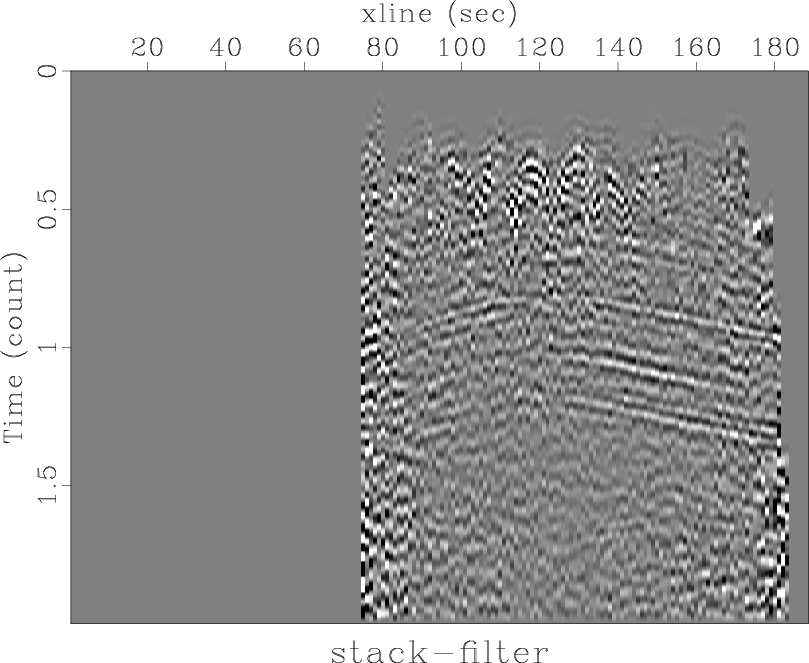
Figure 16 is the final stack with a 20 Hz high cut filter. The maximium frequency in migration was limited to reduce runtime. You can compare Figure 16 to Figure 15 and observe how much signal is lost in order to get a faster runtime.
Figure 17 shows the interval velocity slowness in a 3D cube with depth as the slowest axis. This is the file required to define the velocity to sfzomig3.
Figure 18 shows the real part of the stack data after Fourier transform and transpose to make frequency the slowest axis. This is the file required to define the surface data to sfzomig3.
Figure 19 is the migrated data converted back to time. It can be compared to the commercial migration in Figure 20. One large difference in these results is the commercial migration has zeroed the areas zero on the input stack, a common practice. Another difference is 20 Hz high cut filter applied to limit compute time when creating Figure 19.
|
|---|
|
stack-filter
Figure 16. Final stack with a 20 Hz high cut filter. |
|
|

|
|---|
|
slo
Figure 17. The interval velocity slowness for input to sfzomig3. |
|
|

|
|---|
|
real
Figure 18. The real part of the frequency domain seismic data for input to sfzomig3. |
|
|

|
|---|
|
mig-t
Figure 19. The migrated data. Wavefronts have not been muted from the zero portions of the stack volume. Migration was severely frequency limited to reduce computer time. |
|
|

|
|---|
|
filt-mig
Figure 20. Commercial migration. |
|
|
|
|
|
|
Processing the Teapot Dome Land 3D Survey with Madagascar |