Micro-earthquake monitoring with sparsely-sampled data

Example

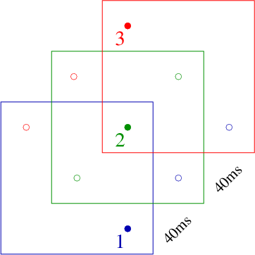
I exemplify the interferometric imaging condition method with a synthetic example simulating the acquisition geometry of the passive seismic experiment performed at the San Andreas Fault Observatory at Depth (Vasconcelos et al., 2008; Chavarria et al., 2003). This numeric experiment simulates waves propagating from three micro-earthquake sources located in the fault zone, Figure 3, which are recorded in a deviated well located at a distance from the fault. For the imaging procedure described in this paper, the micro-earthquakes represent the seismic sources. This experiment uses acoustic waves, corresponding to the situation in which we use the P-wave mode recorded by the three-component receivers located in the borehole, Figures 4(b) and 5(b). The three sources are triggered $40$ ms apart and the triggering time of the second source is conventionally taken to represent the origin of the time axis.

The goal of this experiment is to locate the source positions by focusing data recorded using dense acquisition in media with random fluctuations or by focusing data recorded using sparse acquisition arrays in media without random fluctuations. In the first case, the imaging artifacts are caused by the fact that data are imaged with a velocity model that does not incorporate all random fluctuations of the model used for data simulation, while in the second case, the imaging artifacts are caused by the fact that the data are sampled sparsely in the borehole array. The third case is a combination of acquisition with two sparse arrays, and imaging with an inaccurate velocity model.

meqs Figure 3. Geometry of the sources used in the numeric experiment. The horizontal and vertical separation between sources is $250$ m. The sources are triggered with $40$ ms delays in the order indicated by their numbers. Time ${ t } =0$ is conventionally set to the the triggering moment of source $2$.

wfl3-14,rev3
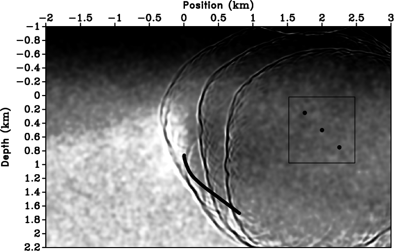
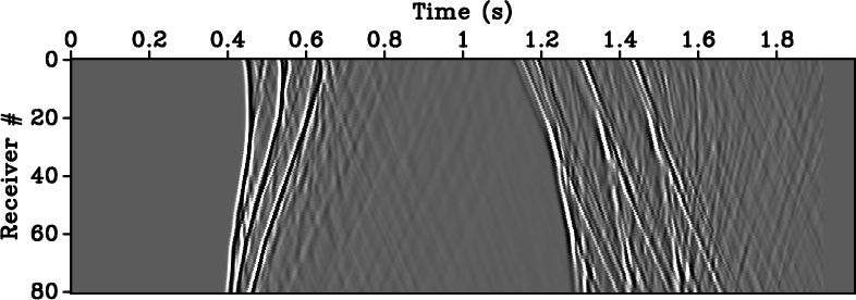
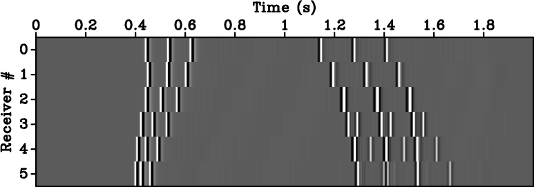
Figure 4. (a) Wavefields simulated in random media and (b) data acquired with a dense receiver array. Overlain on the model and wavefield are the positions of the sources and borehole receivers. The boxed area corresponds to the images depicted in Figures 7(a)-7(b).

wfl4-14,rev4
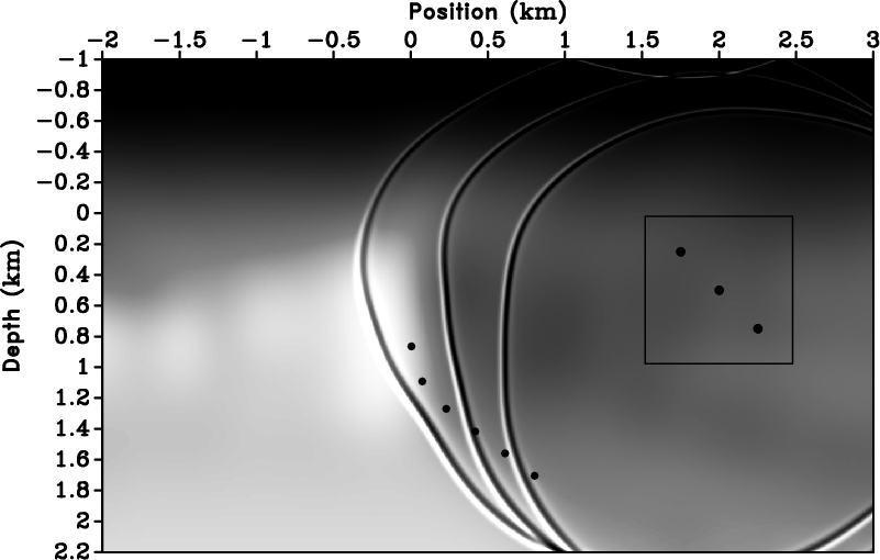
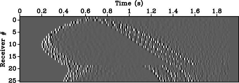
Figure 5. (a) Wavefields simulated in smooth media and (b) data acquired with a sparse receiver array. Overlain on the model and wavefield are the positions of the sources and borehole receivers. The boxed area corresponds to the images depicted in Figures 8(a)-8(b).

wfl3-14,rev3
Figure 6. (a) Wavefields simulated in random media and (b) data acquired with two sparse receiver arrays. Overlain on the model and wavefield are the positions of the sources and borehole receivers. The boxed area corresponds to the images depicted in Figures 9(a)-9(b). The top traces in panel (b) correspond to the vertical array, and the other traces correspond to the sparse deviated array.

uuu3,wig3
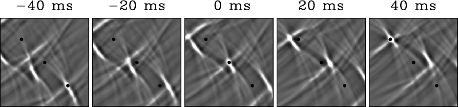
Figure 7. Images corresponding to migration of the densely-sampled data (Figure 4(b)) modeled in the random velocity by (a) conventional I.C. and (b) interferometric I.C. using the background velocity. The left-most panel shows focusing at source $1$, the middle panel shows focusing at source $2$, and the right-most panel shows focusing at source $3$. The overlain dots represent the exact source positions.

uuu4,wig4
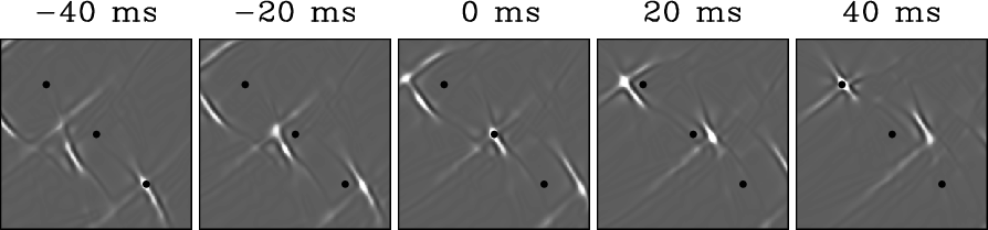
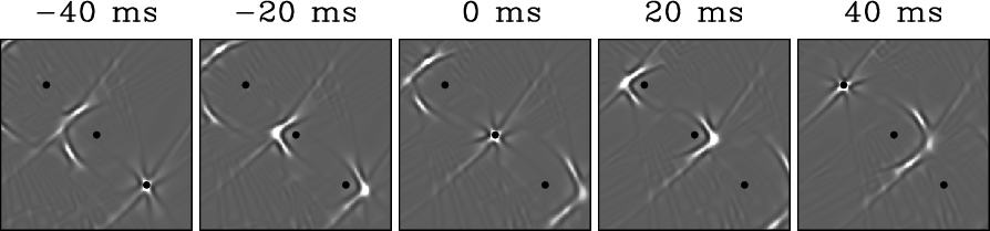
Figure 8. Images corresponding to migration of the sparsely-sampled data (Figure 5(b)) modeled in the background velocity by (a) conventional I.C. and (b) interferometric I.C. using the background velocity. The left-most panel shows focusing at source $1$, the middle panel shows focusing at source $2$, and the right-most panel shows focusing at source $3$. The overlain dots represent the exact source positions.

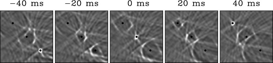
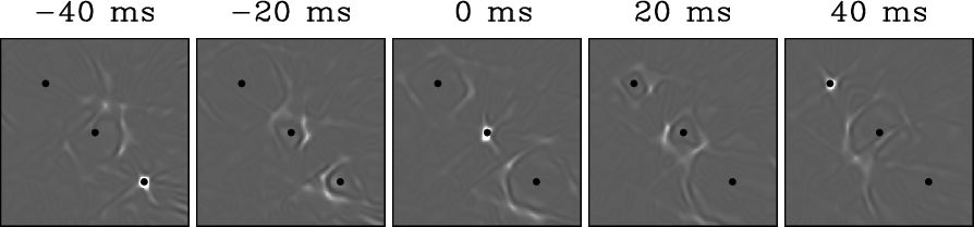
uuu3,wig3
Figure 9. Images corresponding to migration of the dual sparsely-sampled data (Figure 6(b)) modeled in the random velocity by (a) conventional I.C. and (b) interferometric I.C. using the background velocity. The left-most panel shows focusing at source $1$, the middle panel shows focusing at source $2$, and the right-most panel shows focusing at source $3$. The overlain dots represent the exact source positions.

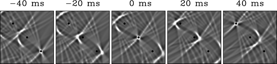
Figures 7(a)-7(b), 8(a)-8(b) and 9(a)-9(b) show the wavefields reconstructed in reverse time around the target location. From left to right, the panels represent the wavefield at different times. As indicated earlier, the time at which source $2$ focuses is selected as time ${ t } =0$, although this convention is not relevant for the experiment and any other time could be selected as reference. The experiment depicted in Figures 7(a)-7(b) corresponds to modeling in a model with random fluctuations and migration in a smooth background model. In this experiment, the data used for imaging are densely-sampled in the borehole, i.e. there are $81$ receivers separated by approximately $12$ m. In contrast, the experiment depicted in 8(a)-8(b) corresponds to modeling and migration in the smooth background model. In this experiment, the data are sparsely-sampled in the borehole, i.e. there are only $6$ receivers obtained by selecting every $16$th receiver from the original set. In all cases, panels (a) correspond to imaging with a conventional imaging condition, i.e. simply select the reconstructed wavefield at various times, and panels (b) correspond to imaging with the interferometric imaging condition, i.e. select various times from the wavefield transformed with a pseudo-WDF of $11$ grid points in space and $5$ grid points in time. For this example, WDF window corresponds to $44$ m in space and $2$ ms in time.

Figure 7(a) shows significant random fluctuations caused by wavefield reconstruction using an inaccurate velocity model. The fluctuations caused by the random velocity and encoded in the recorded data are not corrected during wavefield reconstruction and they remain present in the model. Likewise, Figure 8(a) shows significant random fluctuations caused by reconstruction using the sparse borehole data. However, the pseudo WDF applied to the reconstructed wavefields attenuates the rapid wavefield fluctuations and leads to sparser, better focused images that are easier to use for source location. This conclusion applies equally well for the experiments depicted in Figures 7(a)-7(b) or 8(a)-8(b).

The final example corresponds to the case of acquisition with two separate sparse arrays, Figures 6(a)-6(b). As expected, the wavefields are far less noisy after the application of the WDF, and the focusing is increased due to the larger array aperture. This facilitates an automatic procedure for focusing identification, since most of the spurious noisy is eliminated from the image.

Finally, I note that the 2D imaging results from this example show better focusing than what would be expected in 3D. This is simply because the 1D acquisition in the borehole cannot constrain the 3D location of the micro-earthquakes, i.e. the azimuthal resolution is poor, especially if scatterers are not present in the model used for imaging. This situation can be improved by using data acquired in several boreholes or by using additional information extracted from the wavefields, e.g. polarization of multicomponent data.

Micro-earthquake monitoring with sparsely-sampled data