|
|
|
|
Elastic wave-mode separation for VTI media |
Figure ![]() shows one snapshot of the modeled elastic anisotropic
wavefields using the model shown in Figure 14.
Figure
shows one snapshot of the modeled elastic anisotropic
wavefields using the model shown in Figure 14.
Figure ![]() illustrates the separation of the anisotropic elastic
wavefields using the
illustrates the separation of the anisotropic elastic
wavefields using the
![]() and
and
![]() operators, and
Figure
operators, and
Figure ![]() illustrates the separation using my pseudo
derivative operators. Figure
illustrates the separation using my pseudo
derivative operators. Figure ![]() shows the residual of
unseparated P and S wave modes, such as at coordinates
shows the residual of
unseparated P and S wave modes, such as at coordinates ![]() km and
km and
![]() km in the qP panel and at
km in the qP panel and at ![]() km and
km and ![]() km in the
qS panel. The residual of S waves in the qP panel
of Figure
km in the
qS panel. The residual of S waves in the qP panel
of Figure ![]() is very significant because of strong
reflections from the salt bottom. This extensive residual can be
harmful to under-salt elastic or even acoustic migration, if not
removed completely. In contrast, Figure
is very significant because of strong
reflections from the salt bottom. This extensive residual can be
harmful to under-salt elastic or even acoustic migration, if not
removed completely. In contrast, Figure ![]() shows the
qP and qS modes better separated,
demonstrating the effectiveness of the anisotropic pseudo derivative
operators constructed using the local medium parameters. These
wavefields composed of well separated qP and qS modes are
essential to producing clean seismic images.
shows the
qP and qS modes better separated,
demonstrating the effectiveness of the anisotropic pseudo derivative
operators constructed using the local medium parameters. These
wavefields composed of well separated qP and qS modes are
essential to producing clean seismic images.
In order to test the separation with a homogeneous assumption of
anisotropy in the model, I show in Figure ![]() the
separation with
the
separation with
![]() and
and
![]() in the
in the ![]() domain. This separation assumes a model with homogeneous
anisotropy. The separation shows that there is still residual in the
separated panels. Although the residual is much weaker compared to
separating using an isotropic model, it is still visible at locations
such as at coordinates
domain. This separation assumes a model with homogeneous
anisotropy. The separation shows that there is still residual in the
separated panels. Although the residual is much weaker compared to
separating using an isotropic model, it is still visible at locations
such as at coordinates ![]() km and
km and ![]() km, and
km, and ![]() km and
km and
![]() km in the qP panel and at
km in the qP panel and at ![]() km and
km and ![]() km in the
qS panel.
km in the
qS panel.


|
|---|
|
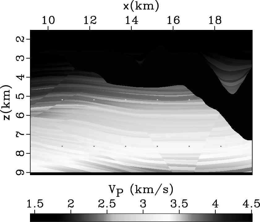
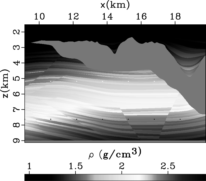
vp,vs,ro,epsilon,delta
Figure 14. A Sigsbee 2A model in which (a) is the P wave velocity (taken from the original Sigsbee 2A model (Paffenholz et al., 2002) ), (b) is the S wave velocity, where |
|
|

|
|---|
|
uA-f24-wom
Figure 15. Anisotropic wavefield modeled with a vertical point force source at |
|
|

|
|---|
|
qA-f24-wom
Figure 16. Anisotropic qP and qS modes separated using |
|
|

|
|---|
|
pA-f24-wom
Figure 17. Anisotropic qP and qS modes separated using pseudo derivative operators for the vertical and horizontal components of the elastic wavefields shown in Figure |
|
|

|
|---|
|
mA-f24-wom
Figure 18. Anisotropic qP and qS modes separated in the |
|
|
|
|
|
|
Elastic wave-mode separation for VTI media |