|
|
|
|
Interferometric imaging condition for wave-equation migration |
For all our examples, we extrapolate wavefields using time-domain
finite-differences both for modeling and for migration. Thus, we
simulate a reverse-time imaging procedure, although the theoretical
results derived in this paper apply equally well to other wavefield
reconstruction techniques, e.g. downward continuation, Kirchhoff
integral methods, etc. The parameters used in our examples, explained
in Appendix A, are: seismic spatial wavelength ![]() m,
wavelet central frequency
m,
wavelet central frequency ![]() Hz, random fluctuations
parameters:
Hz, random fluctuations
parameters: ![]() m,
m, ![]() m,
m, ![]() , and random noise
magnitude
, and random noise
magnitude ![]() .
.
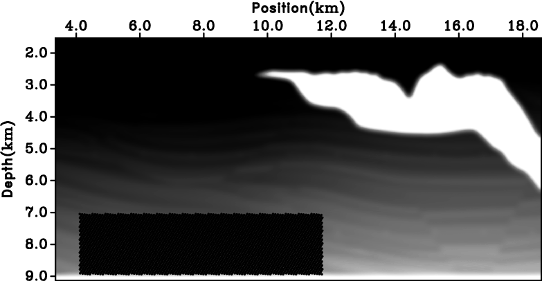
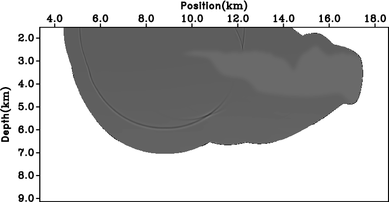
Consider the model depicted in Figures 10(a)-10(d).
As in the preceding example, the left panels depict the known smooth
velocity ![]() , and the right panels depict the model with random
variations. The imaging target is represented by the oblique lines,
Figure 9(b), located around
, and the right panels depict the model with random
variations. The imaging target is represented by the oblique lines,
Figure 9(b), located around ![]() km, which simulates a
cross-section of a stratigraphic model.
km, which simulates a
cross-section of a stratigraphic model.
We model data with a random velocity model and image using the smooth
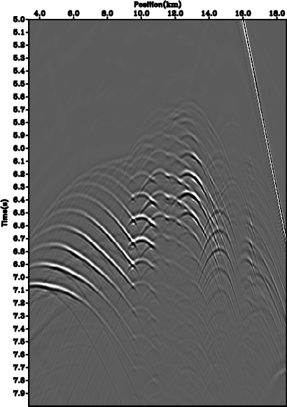
model. Figures 10(a)-10(d) show wavefield snapshots
in the two models for different propagation times, one before the
source wavefields interact with the target reflectors and one after
this interaction. The propagating waves are affected the the random
fluctuations in the model both before and after their interaction with
the reflectors. Figures 10(e) and 10(f) show the
corresponding recorded data on the acquisition surface located at
![]() , where
, where ![]() represents the wavelength of the source
pulse.
represents the wavelength of the source
pulse.
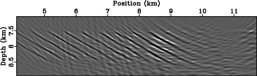
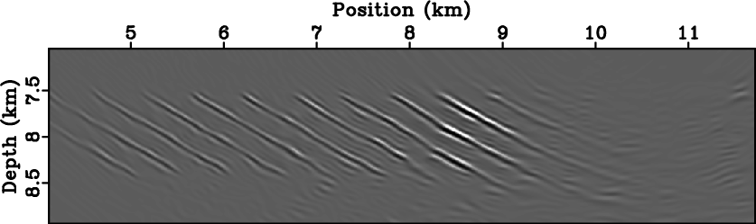
Migration with a conventional imaging condition of the data simulated in the background model using the same velocity produces the image in Figure 11(a). The targets are well imaged, although the image also shows artifacts due to truncation of the data on the acquisition surface. In contrast, migration with the conventional imaging condition of the data simulated in the random model using the background velocity produces the image in Figure 11(b). This image is distorted by the random variations in the model that are not accounted for in the background migration velocity. The targets are harder to discern since they overlap with many truncation and defocusing artifacts caused by the inaccurate migration velocity.
Finally, Figure 11(c) shows the migrated image using the interferometric imaging condition applied to the wavefields reconstructed in the background model from the data simulated in the random model. Many of the artifacts caused by the inaccurate velocity model are suppressed and the imaging targets are more clearly visible and easier to interpret. Furthermore, the general patterns of amplitude variation along the imaged reflectors are similar between Figures 11(b) and 11(c).
We note that the reflectors are not as well imaged as the ones obtained when the velocity is perfectly known. This is because the interferometric imaging condition described in this paper does not correct kinematic errors due to inaccurate velocity. It only acts on the extrapolated wavefields to reduce wavefield incoherency and add statistical stability to the imaging process. Further extensions to the interferometric imaging condition can improve focusing and enhance the images by correcting wavefields prior to imaging. However, this topic falls outside the scope of this paper and we do not elaborate on it further.

|
|---|
|
avo,xm
Figure 9. Velocity model (a) and imaging target located around |
|
|


|
|---|
|
awo-5,awv-5,awo-7,awv-7,ado,adv
Figure 10. Seismic snapshots of acoustic wavefields simulated in the background velocity model (a)-(c), and in the random velocity model (b)-(d). Data recorded at the surface from the simulation in the background velocity model (e) and from the simulation in the random velocity model (f). |
|
|

|
|---|
|
winacic0,winacic1,winaiic1
Figure 11. Image produced using the conventional imaging condition from data simulated in the background model (a) and from data simulated in the random model (b). Image produced using the interferometric imaging condition from data simulated in the random model (c). |
|
|
|
|
|
|
Interferometric imaging condition for wave-equation migration |