|
|
|
|
Interferometric imaging condition for wave-equation migration |
Consider the complex signal
![]() which depends on time
which depends on time
![]() . By definition, its Wigner distribution function (WDF)
is (Wigner, 1932):
. By definition, its Wigner distribution function (WDF)
is (Wigner, 1932):
A special subset of the transformation equation C-1 corresponds to zero
temporal frequency. For input signal
![]() , we obtain the
output Wigner distribution function
, we obtain the
output Wigner distribution function
![]() as
as
The WDF transformation can be generalized to multi-dimensional signals
of space and time. For example, for 2D real signals function of space,
![]() , the zero-wavenumber pseudo WDF can be formulated as
, the zero-wavenumber pseudo WDF can be formulated as
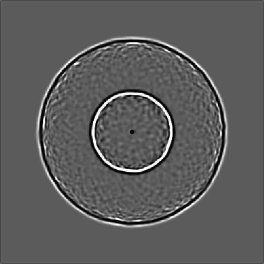
For illustration, consider the model depicted in Figure 1(a). This
model consists of a smoothly-varying background with ![]() random
fluctuations. The acoustic seismic wavefield corresponding to a source
located in the middle of the model is depicted in
Figure 1(b). This wavefield snapshot can be considered as the
random ``image''. The application of the 2D pseudo WDF transformation
to images shown in Figure 1(b) produces the image shown in
Figure 1(c). We can make three observations on this image:
first, the random noise is strongly attenuated; second, the output
wavelet is different from the input wavelet, as a result of the
bi-linear nature of the pseudo WDF transformations; third, the
transformation is isotropic, i.e. it operates identically in all
directions. The pseudo WDF applied to this image uses
random
fluctuations. The acoustic seismic wavefield corresponding to a source
located in the middle of the model is depicted in
Figure 1(b). This wavefield snapshot can be considered as the
random ``image''. The application of the 2D pseudo WDF transformation
to images shown in Figure 1(b) produces the image shown in
Figure 1(c). We can make three observations on this image:
first, the random noise is strongly attenuated; second, the output
wavelet is different from the input wavelet, as a result of the
bi-linear nature of the pseudo WDF transformations; third, the
transformation is isotropic, i.e. it operates identically in all
directions. The pseudo WDF applied to this image uses ![]() grid points in the vertical and horizontal directions. As indicated in
the body of the paper, we do not discuss here the optimal selection of
the WDF window. Further details of Wigner distribution functions and
related transformations are discussed by
Cohen (1995).
grid points in the vertical and horizontal directions. As indicated in
the body of the paper, we do not discuss here the optimal selection of
the WDF window. Further details of Wigner distribution functions and
related transformations are discussed by
Cohen (1995).


|
|---|
|
ss,wfl-6,wdf-6
Figure 12. Random velocity model (a), wavefield snapshot simulated in this model by acoustic finite-differences (b), and its 2D pseudo Wigner distribution function (c). |
|
|
|
|
|
|
Interferometric imaging condition for wave-equation migration |