|
 |
 |
 | Stereographic imaging condition for wave-equation migration |  |
![[pdf]](icons/pdf.png) |
Next: Example
Up: Sava: Stereographic imaging
Previous: Conventional imaging condition
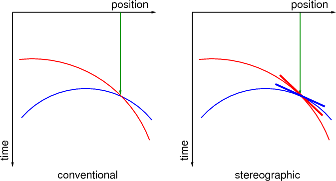
One possibility to remove the artifacts caused by the cross-talk
between inconsistent reflection events is to modify the imaging
condition to use more than one attribute for matching the source and
receiver wavefields. For example, we could use the time and slope to
match events in the wavefield, thus distinguishing between unrelated
events that occur at the same time (Figure 4).
|
|---|
stereo2
Figure 4. Comparison of
conventional imaging (a) and stereographic imaging (b).
|
|---|
![[png]](icons/viewmag.png) ![[xfig]](icons/xfig.png)
|
|---|
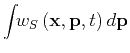
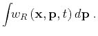
A simple way of decomposing the source and receiver wavefields
function of local slope at every position and time is by local
slant-stacks at coordinates  and
and  in the four-dimensional
source and receiver wavefields. Thus, we can write the total source
and receiver wavefields (
in the four-dimensional
source and receiver wavefields. Thus, we can write the total source
and receiver wavefields ( and
and  ) as a sum of decomposed
wavefields (
) as a sum of decomposed
wavefields ( and
and  ):
):
Here, the three-dimensional vector  represents the local
slope function of position and time. Using the wavefields decomposed
function of local slope, and , we can design a
stereographic imaging condition which cross-correlates the wavefields
in the decomposed domain, followed by summation over the decomposition
variable:
represents the local
slope function of position and time. Using the wavefields decomposed
function of local slope, and , we can design a
stereographic imaging condition which cross-correlates the wavefields
in the decomposed domain, followed by summation over the decomposition
variable:
 |
(7) |
Correspondence between the slopes p of the decomposed source and
receiver wavefields occurs only in planes dipping with the slope of
the imaged reflector at every location in space. Therefore, an
approximate measure of the expected reflector slope is required for
correct comparison of corresponding reflection data in the decomposed
wavefields. The choice of the word ``stereographic'' for this imaging
condition is analogous to that made for the velocity estimation method
called stereotomography (Billette et al., 2003; Billette and Lambare, 1997) which
employs two parameters (time and slope) to constrain traveltime
seismic tomography.
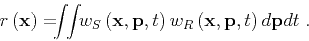
For comparison with the stereographic imaging condition 7, the
conventional imaging condition can be reformulated using the wavefield
notation 5-6 as follows:
![\begin{displaymath}
r\left ({ \bf x}\right)=
\!\!\!\int\!\! \left [\int\!\! w_...
..._R\left ({ \bf x},{ \bf p},t \right) d{ \bf p} \right] dt \;.
\end{displaymath}](img31.png) |
(8) |
The main difference between imaging conditions 7 and
8 is that in one case we are comparing independent slope
components of the wavefields separated from one-another, while in the
other case we are comparing a superposition of them, thus not
distinguishing between waves propagating in different directions.
This situation is analogous to that of reflectivity analysis function
of scattering angle at image locations, in contrast with reflectivity
analysis function of acquisition offset at the surface. In the first
case, waves propagating in different directions are separated from
one-another, while in the second case all waves are superposed in the
data, thus leading to imaging artifacts (Stolk and Symes, 2004).
Figure 3(b) shows the image produced by stereographic imaging of
the data generated for the model depicted in
Figures 1(a)-1(b), and Figure 5(b) shows the
similar image for the model depicted in
Figures 2(a)-2(b). Images 3(b) and
5(b) use the same source receiver wavefields as images
3(a) and 5(a), respectively. In both cases, the
cross-talk artifacts have been eliminated by the stereographic imaging
condition.

|
|---|
ii,kk
Figure 5.
Images obtained for the model in Figures 2(a)-2(c)
using the conventional imaging condition (a) and the stereographic
imaging condition (b).
|
|---|
![[scons]](icons/configure.png)
|
|---|


|
|---|
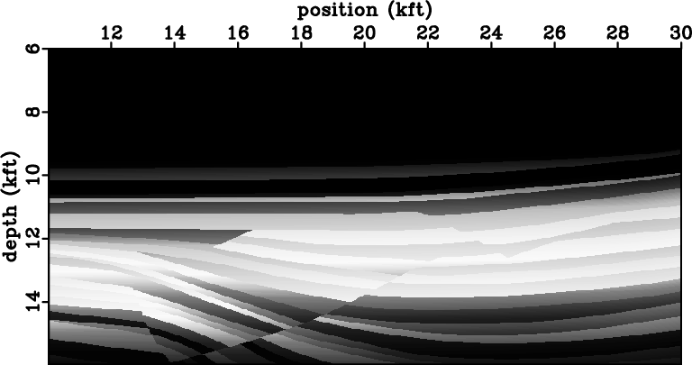
ttr1,ii1,ttr2,ii2,ttr0,ii0,vel,kk
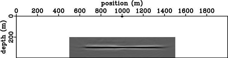
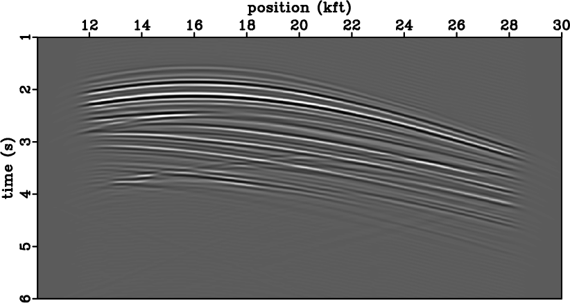
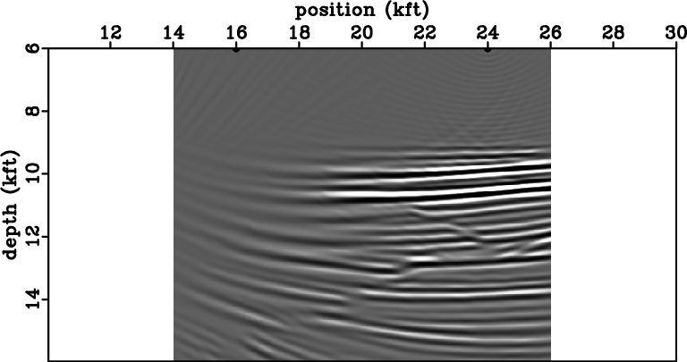
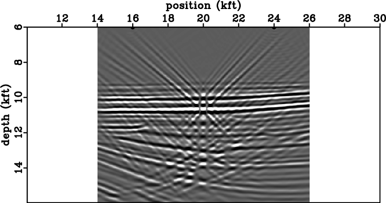
Figure 6. Data corresponding to shots located at coordinates  kft (a), kft (a),
 kft (c), and the sum of data corresponding to both shot
locations (e). Image obtained by conventional imaging condition for
the shots located at coordinates kft (b), kft (d) and
the sum of data for both shots (f). Velocity model extracted from the
Sigsbee 2A model (g) and image from the sum of the shots located at
kft and kft obtained using the stereographic imaging
condition (h). kft (c), and the sum of data corresponding to both shot
locations (e). Image obtained by conventional imaging condition for
the shots located at coordinates kft (b), kft (d) and
the sum of data for both shots (f). Velocity model extracted from the
Sigsbee 2A model (g) and image from the sum of the shots located at
kft and kft obtained using the stereographic imaging
condition (h).
|
|---|
|
|
|---|
|
|
|
|
| Stereographic imaging condition for wave-equation migration | |
|
Next: Example
Up: Sava: Stereographic imaging
Previous: Conventional imaging condition
2013-08-29