|
|
|
|
Random noise attenuation using |
|
|---|
|
para,npara,tpefpatch,fxpatch,npre,npar
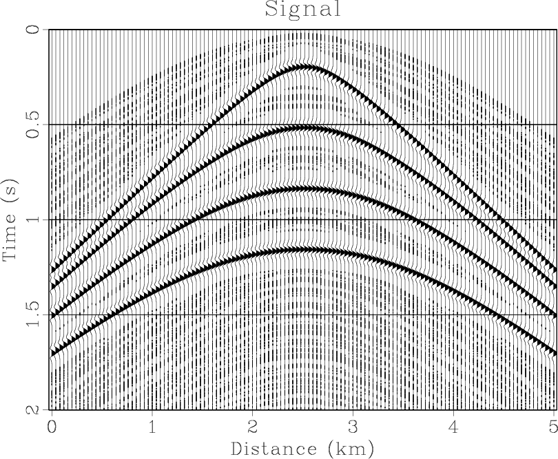
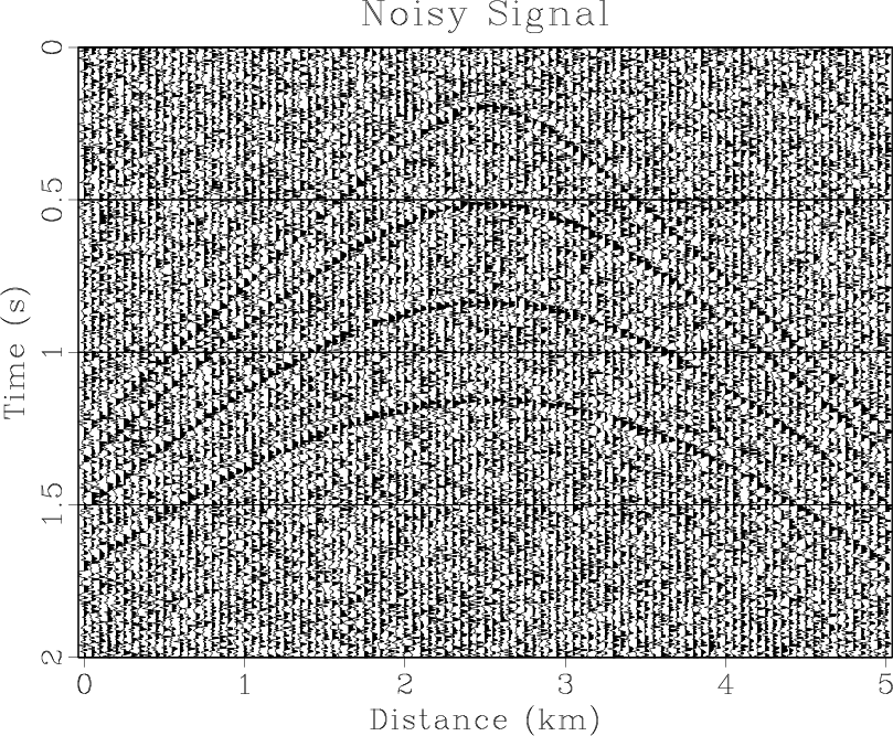
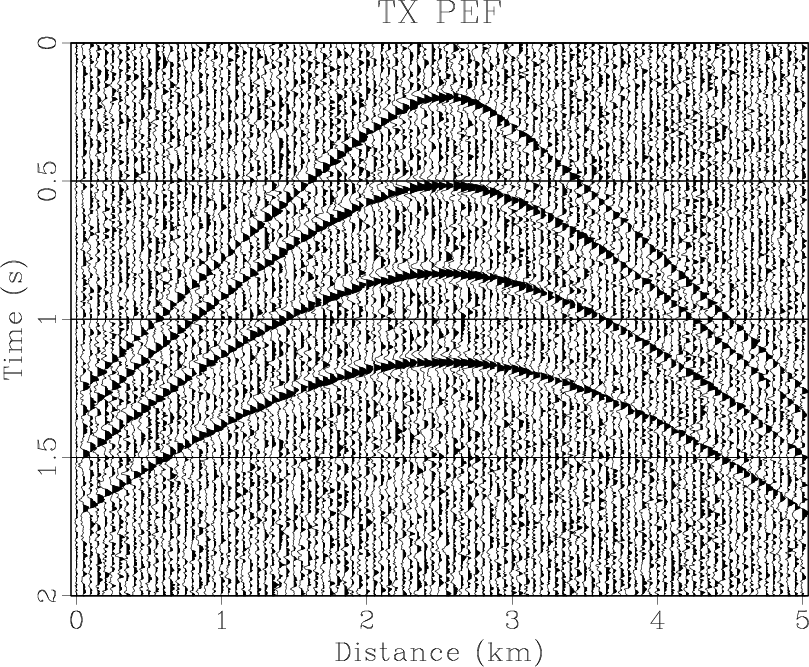
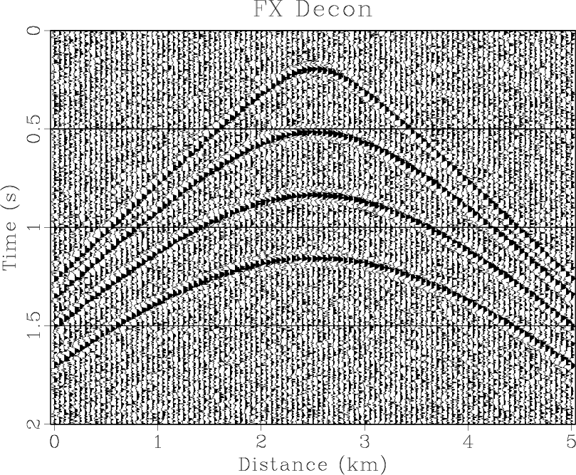
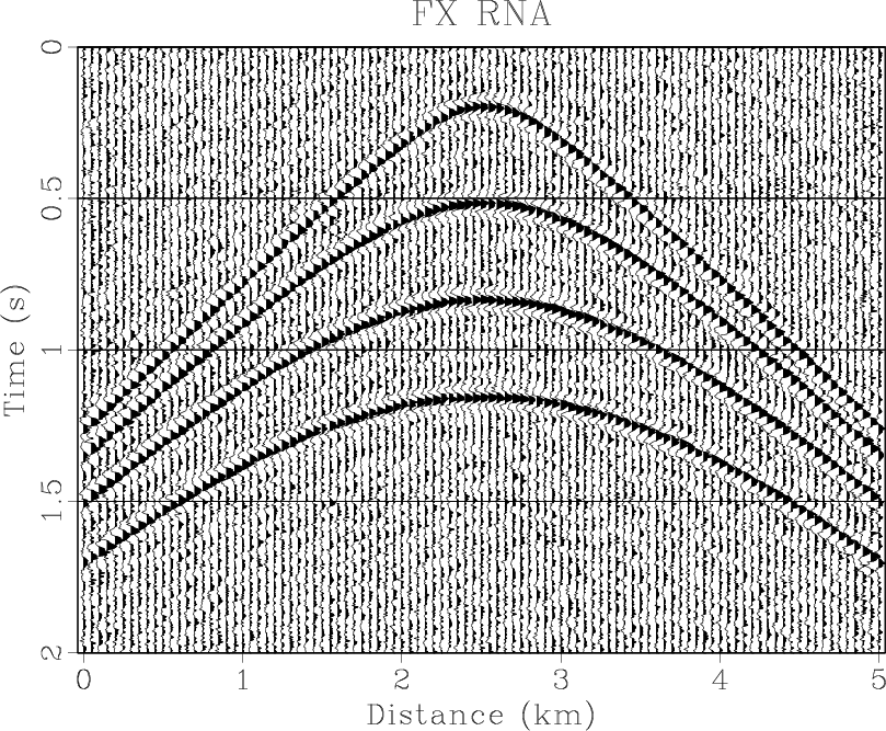
Figure 4. (a) Synthetic shot gather. (b) Noisy gather. (c) Result of |
|
|
|
|---|
|
fxdiff,mpapatch,ndiff
Figure 5. Difference sections of |
|
|
Figure 4(a) shows a synthetic shot gather with four hyperbolic events,
501 traces. Some random noise is added to this gather. We do not use windows in time
for this example. For ![]() -
-![]() RNA, the length of filter is
RNA, the length of filter is ![]() and the smoothing radiuses in
space and frequency axes are respectively 20 and 3,
and the smoothing radiuses in
space and frequency axes are respectively 20 and 3, ![]() ,
, ![]() . The
. The ![]() -
-![]() domain prediction
is implemented over a sliding window of 20 traces width with 50% overlap and the filter length is 6,
domain prediction
is implemented over a sliding window of 20 traces width with 50% overlap and the filter length is 6, ![]() and
the
and
the ![]() -
-![]() domain prediction is implemented over the same sliding window and the filter length in space and
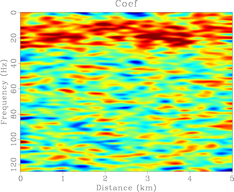
time are 6 and 5 respectively. The estimated nonstationary coefficients by the proposed
domain prediction is implemented over the same sliding window and the filter length in space and
time are 6 and 5 respectively. The estimated nonstationary coefficients by the proposed ![]() -
-![]() RNA are shown
in Figure 4(f). Note that the middle coefficient is bigger than the sideward, which is because the dip of
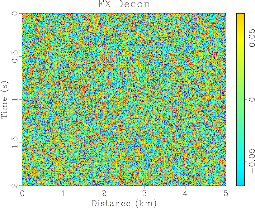
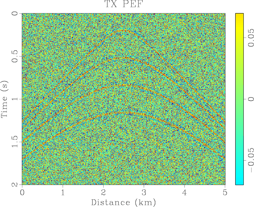
the middle is smaller than the sideward. The results of three methods are shown in Figures 4(d)- 6(d),
respectively. The
RNA are shown
in Figure 4(f). Note that the middle coefficient is bigger than the sideward, which is because the dip of
the middle is smaller than the sideward. The results of three methods are shown in Figures 4(d)- 6(d),
respectively. The ![]() -
-![]() RNA achieves a similar result to
RNA achieves a similar result to ![]() -
-![]() domain and
domain and ![]() -
-![]() domain prediction methods.
However, we use equation 11 to compute the SNRs of the results of three methods. The SNRs of three
methods are 0.98 dB, 1.25 dB, 1.67 dB, respectively. The
domain prediction methods.
However, we use equation 11 to compute the SNRs of the results of three methods. The SNRs of three
methods are 0.98 dB, 1.25 dB, 1.67 dB, respectively. The ![]() -
-![]() RNA can improve SNR more greatly. The
RNA can improve SNR more greatly. The
![]() -
-![]() RNA solves the nonstationary case by allowing the coefficients smoothly varying, while
RNA solves the nonstationary case by allowing the coefficients smoothly varying, while ![]() -
-![]() domain
or
domain
or ![]() -
-![]() domain prediction method uses windowing strategies. From the difference sections (Figure 7(a)- 5(c)), we
find that
domain prediction method uses windowing strategies. From the difference sections (Figure 7(a)- 5(c)), we
find that ![]() -
-![]() domain and
domain and ![]() -
-![]() domain prediction methods damage more signals than
domain prediction methods damage more signals than ![]() -
-![]() RNA. If we use
windows in time for this example, we can obtain better results. This example shows that
RNA. If we use
windows in time for this example, we can obtain better results. This example shows that ![]() -
-![]() RNA can
be used for random noise attenuation in shot gather.
RNA can
be used for random noise attenuation in shot gather.
|
|
|
|
Random noise attenuation using |