|
 |
 |
 | Imaging in shot-geophone space |  |
![[pdf]](icons/pdf.png) |
Next: THE MEANING OF THE
Up: SURVEY SINKING WITH THE
Previous: The DSR equation in
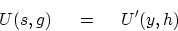
By converting the DSR equation to midpoint-offset space
we will be able to identify the familiar zero-offset migration part
along with corrections for offset.
The transformation between  recording parameters
and
recording parameters
and  interpretation parameters is
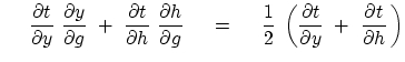
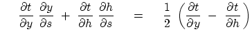
Travel time  may be parameterized in -space or -space.
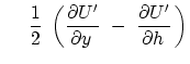
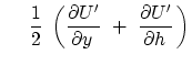
Differential relations for this
conversion are given by the chain rule for derivatives:
may be parameterized in -space or -space.
Differential relations for this
conversion are given by the chain rule for derivatives:
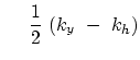
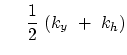
Having seen how stepouts transform from shot-geophone space
to midpoint-offset space,
let us next see that spatial frequencies transform in much the same way.
Clearly, data could be transformed from  -space
to -space with (9.15) and (9.16)
and then Fourier transformed to
-space
to -space with (9.15) and (9.16)
and then Fourier transformed to  -space.
The question is then,
what form would the double-square-root equation (9.13)
take in terms of the spatial frequencies ?
Define the seismic data field in either coordinate system as
-space.
The question is then,
what form would the double-square-root equation (9.13)
take in terms of the spatial frequencies ?
Define the seismic data field in either coordinate system as
 |
(19) |
This introduces a new mathematical function  with the same
physical meaning as
with the same
physical meaning as  but,
like a computer subroutine or function call,
with a different subscript look-up procedure
for than for .
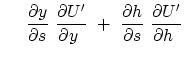
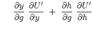
Applying the chain rule for partial differentiation to (9.19) gives
but,
like a computer subroutine or function call,
with a different subscript look-up procedure
for than for .
Applying the chain rule for partial differentiation to (9.19) gives
and utilizing (9.15) and (9.16) gives
In Fourier transform space
where
 transforms to
  ,
equations (9.22) and (9.23),
when
,
equations (9.22) and (9.23),
when  and
and  are cancelled, become
Equations (9.24)
and (9.25)
are Fourier representations of (9.22) and (9.23).
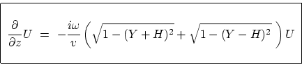
Substituting (9.24) and (9.25)
into (9.13) achieves the main purpose of this section,
which is to get the double-square-root migration equation
into midpoint-offset coordinates:
![\begin{displaymath}
{\partial \over \partial z} U = - i
{\omega \o...
...y - v k_h \over 2 \omega } \right)^2
} \right] U
\end{displaymath}](img93.png) |
(26) |
Equation (9.26) is the takeoff point
for many kinds of common-midpoint seismogram analyses.
Some convenient definitions that simplify its appearance are
The new definitions  and
and  are the sines
of the takeoff angle and of the arrival angle of a ray.
When these sines are at their limits of
are the sines
of the takeoff angle and of the arrival angle of a ray.
When these sines are at their limits of  they refer
to the steepest possible slopes in
they refer
to the steepest possible slopes in  - or
- or  -space.
Likewise,
-space.
Likewise,  may be interpreted as the dip of the data as seen
on a seismic section.
The quantity
may be interpreted as the dip of the data as seen
on a seismic section.
The quantity  refers to stepout observed on a common-midpoint gather.
With these definitions (9.26) becomes slightly less cluttered:
refers to stepout observed on a common-midpoint gather.
With these definitions (9.26) becomes slightly less cluttered:
 |
(31) |
EXERCISES:
- Adapt equation (9.26) to allow for a difference in velocity
between the shot and the geophone.
- Adapt equation (9.26) to allow for downgoing pressure waves
and upcoming shear waves.
|
|
|
|
| Imaging in shot-geophone space | |
|
Next: THE MEANING OF THE
Up: SURVEY SINKING WITH THE
Previous: The DSR equation in
2009-03-16